Download
1 / 84
860 likes | 982 Views
A Practical Overview of Structural Equation Modeling for Business Research. Key Sources. Lecture notes from: Todd Boyle, Winston Jackson, Norine Verberg (StFX) Gordon Stringer (UCCS) Lydia Miljan, (University of Windsor) Johnny Amora (De la Salle-College of Saint Benilde)

E N D
A Practical Overview of Structural Equation Modeling for Business Research
Key Sources • Lecture notes from: • Todd Boyle, Winston Jackson, Norine Verberg (StFX) • Gordon Stringer (UCCS) • Lydia Miljan, (University of Windsor) • Johnny Amora (De la Salle-College of Saint Benilde) • Falk, R. F. & Miller, N. B. (1992), A Primer for soft modeling. Akron, Ohio, The University of Akron Press. • Hulland J. (1999), Use of partial least squares (PLS) in strategic management research: A review of four recent studies. Strategic Management Journal, 20(2), pp. 195 – 204.
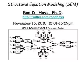
Path Analysis Path analysis is an extension of regression In path analysis the researcher is examining the ability of more than one predictor variable to explain or predict multiple dependent variables
Manifest Variables • Variables that the researcher has observed or measured • In all diagrams, measured variables are depicted by squares or rectangles • In path analysis, all variables are measured
Exogenous / Independent Variables A variable in a model that is not affected by another variable in the model In this path analysis, there are two exogenous/ independent variables: X1 and X2
Endogenous / Dependent Variables A variable in a model that is affected by another variable in the model In this path analysis, there are two endogenous variables: Y1 and Y2
Direct Effects • Those parameters that estimate the direct effect one variable has on another • These are indicated by the arrows that are drawn from one variable to another • In this model, four direct effects are measured
Indirect Effects • Indirect effects are those influences that one variable may have on another that is mediated through a third variable • In this model, X1 and X2 have a direct effect on Y1 and indirect effect on Y2 through Y1
Errors in Prediction • As in any prediction model, errors in prediction always exist • Thus, Y1 and Y2 will have errors in prediction
What is AMOS? (Analysis of Moment Structures) • Amos is an easy to use program that tests relationships among observed and latent variables and uses those models to test the hypotheses and confirm relationships • Graphical language - no need to write equations or type commands • Easy to learn-user-friendly features such as drawing tools, configurable toolbars, and drag and drop capabilities • Fast- models that once took days to compute are now completed in seconds
Steps for Performing Path Analysis in AMOS • Replace missing values or eliminate cases in SPSS • Create a new project in AMOS & link SPSS dataset • Build the input path analytic model • Run the model • Examine the goodness-of-fit statistics • Rebuild the model (go to step 4) • Trim the model (go to step 4) • Repeat 6 and 7 until: • Adequate fit is achieved (i.e., good GOF values) • No other model trimming / rebuilding can take place • Present final model and draw conclusions
PA Case 1 • Pilot conducted in 2008 • Determinants of pharmacy staff satisfaction regarding their process for reporting medication errors • Online survey conducted with pharmacist, managers, and support staff: • We will discuss the implications of this later • Simple case to highlight steps of path analysis
Step 1 – Replace Missing Values /Eliminate Cases • Open Dataset: • PA-Case1-Unclean.sav • Examine data • Decide how to replace missing values and/or eliminate specific cases • Save the dataset, with a new name • Exit SPSS
Step 2 – New Project in AMOS & Link SPSS Dataset • Open AMOS • Create a new project • Import / link SPSS Dataset • For consistency, will all use the same clean dataset: • PA-Case1-Clean.sav
Step 3 – Build the InputPath Analytic Model • Create the input path analytic model: • Add the manifest independent, dependent, and intervening variables from the SPSS dataset • Create the paths • Add error terms to the dependent variables • Select standardized data option • Select MI = 4 option (we will discuss this in a little while)
Step 5 – Examine Goodness-of-fit Statistics • Goodness-of-fit (GOF) tells us how well our model fits our data • The better the model fit, the better the predictive capability of the model, and thus the better the model quality • Examples of good and bad model fit • Many different GOF statistics exist: • For now, we are only interested in chi-square and RMSEA
Chi-Square GOF Statistic • Tests the hypothesis that the saturated model (i.e., the model with all possible relationships specified. like q16f to Q17B is possible relationship ) does as good or better job of predicting than your default model (i.e., your conceptual model with only relationships based on theory specified): • If we find significance (i.e., p <= .05), then our model does not fit the data well • We want non-significance (i.e., p > .05)
Chi-Square GOF Statistic • If we look at the probability level on the previous slide we see: • Probability level = .000 • Therefore our model does not fit the data well • However, for large sample sizes this GOF statistic may not hold, therefore we must also check RMSEA
RMSEA • Root mean square error of approximation: • One of the most popular GOF statistics • Takes into consideration model complexity • Among the least impacted by low sample sizes • RMSEA <= 0.05 indicates a good model fit: • The closer to RMSEA = .000, the better the model fit
RMSEA • As you can see from the last slide, the RMSEA for our model (default) is: • Default model = .272 • As this is greater than .05, we can conclude that our model does not fit the data very well • Therefore, we have a poor/low quality model
Model Rebuilding and Trimming • Despite having low GOF for our model, all is not lost • In most cases your initial model will have low GOF • AMOS provides us with new information that we can use to rebuild the model
Revise the Model • Adding important plausible/research justified relationships that we may have missed in the initial model: • This is known as model re-specification or rebuilding • Step 6 • Removing paths that are not statistically significant: • This is known as model trimming • Step 7