Download
1 / 33
330 likes | 339 Views
Combining Argo Data with Other in Situ and Remote Observations Judith Gray U.S. Department of Commerce National Oceanic and Atmospheric Administration Atlantic Oceanographic and Meteorological Laboratory, Miami, FL. Objectives of Large-Scale Ocean Observations.

E N D
Combining Argo Data with Other in Situ and Remote Observations Judith Gray U.S. Department of Commerce National Oceanic and Atmospheric Administration Atlantic Oceanographic and Meteorological Laboratory, Miami, FL
Objectives of Large-Scale Ocean Observations • Provide basic description of physical state of the ocean including variability on seasonal and longer time scales • Reveal processes that influence climate • Provide large-scale context for regional process studies of shorter duration • Produce required data for assimilation and (seasonal and longer) model initialization • Complement satellite remote sensing with data for validation, calibration, and interpretation
Other Global Observing Systems • World Ocean Circulation Experiment (WOCE) repeat deep hydrography • Time Series stations, both buoys and ships • Surface drifter network • Broad-scale XBT network, repeat sections; hi-res XBT/XCTD • Sea-level network (GLOSS calibration & maintenance stndrds • Acoustic tomography/thermography • New technologies: gliders and other autonomous vehicles, addition of compatible biogeochemical sensors, co-evolution with models to enable full integration • NASA/South Africa Satellite Laser Ranging Station - optical radar, part of the international SLR tracking network
Research/Operations Interface • For implementation and maintenance of a complete observing system, a strong partnership between research institutions and operational agencies must be created • Strong leadership and participatory roles on both sides • Integration across Observing System platforms • Integration across instrument development, network design,implementation, data management, scientific analysis, & data assimilation
Co-evolution of Observations and Modeling The roles of observations must be to: • Provide appropriate data and statistics for data assimilation and model initialization, • Provide independent information for testing model results and model processes, and • Discover new phenomena not anticipated in models, thereby stimulating model improvements. The role of models must be to: • Direct enhancements to the observing system, what needs to be measured and where • Use/assimilate the data to improve weather and climate forecasts
Argo Floats Positions of the floats that have delivered data within the last 30 days
ARGO Floats used to Validate Upper Ocean Heat Content Fields Derived from Satellite Altimetry
Upper Ocean Heat Content for Hurricane Studies We compute the upper ocean heat content for hurricane studies. The global field of heat content to the depth of the 26oC isotherm is shown at the top. These fields are computed using altimetry observations. Satellite altimetry measures the sea height, which is proportional to the upper ocean heat content. The higher the sea level, the warmer the upper ocean usually is. Data from ARGO floats are used to validate these estimates. The lower panels show where the validations are done in the maps and the scattered plots show you the error of the estimates. The correlation between the estimates and actual observations is approximately 0.9.
XBT Transects AOML deploys approximately 10,000 XBTs per year in all basins and in different modes (high density (HD)= 4 transects per year, 30 drops per day during the transect; low density (LD) = 12 times per year, 4 drops per day during the transect). High density mode is done mainly to study mesoscale ocean features and currents, while low density are done to investigate large scale – long period ocean variability. Some transects are maintained exclusively by AOML, others in collaboration with international partners. The map shows these transects. AX15 crosses the Gulf of Guinea. It will be done with AOML XBTs with the logistical support of IRD/France.
Quality Controlled Drifting Buoy Observations Nov 1989-early 2006: 887 drifters in S. Atlantic (826 with drogues to Measure mixed-layer currents 688 drifter-years of data
Animations of monthly mean currents and SST from drifters (time mean field shown here)
Monitoring Currents in Real-Time http://www.aoml.noaa.gov/phod/altimetry/cvar/index.php
Surface Currents Surface Currents can be monitored in near-real time (2 day delay) using sea height anomalies derived from altimetry. NOAA/AOML is currently developing web pages that show time series of the variability of several currents, such as the Agulhas Current, the North Brazil Current, the Yucatan Current, and the Florida Current. The figure at the top shows the time series of the transport of the Agulhas Current (across the transect shown in the map in the left) since 1993. This time series is updated once a month. The small circles indicate annual mean values. The figure at the bottom right shows a space time diagram of the sea height anomaly values along a corridor of 5 degrees wide parallel to the coast of South Africa. The high values (reds) indicate warm rings transporting warm and salty waters from the Indian into the Atlantic Ocean.
Access CoastWatch Global Satellite Data and Products Joaquin Trinanes and Gustavo Goni
CoastWatch Products SST Anomalies: View 5-day (pentad) SST anomaly maps for the Caribbean Region. Spatial resolution is 9.28 km. Atlantic SST maps: Display and retrieve daily and pentad Sea Surface Temperature maps for the Atlantic Ocean. These maps are created using data from the POES satellites. Near Real Time Wind Data: Display and retrieve surface wind data from a variety of sensors (QuikSCAT, SSMI, TMI, ERS-2, TOPEX, Jason-1, GFO and Drifters Upper Ocean Heat Content: Upper ocean thermal structure derived from the Sea Surface Height and Sea Surface Temperature fields. Updated daily.
Relevant publication: Enfield, D.B., and L. Cid-Serrano, 2006: Secular and multidecadal warmings in the North Atlantic and their relationships with major hurricanes. Geophys. Res. Lett. Submitted. Is the AMO a Natural Climate Mode and How Does it Affect Hurricanes? David Enfield NOAA Atlantic Oceanographic & Meteorological Lab Miami, Florida Luis Cid-Serrano Dept. Statistics, Universidad de Concepción, Chile
Global warming model w/ greenhouse gases & solar forcing (red) • …residual fluctuations (blue) not explained by GHGs (red) • …implies that residual reflects natural fluctuations in SST NOAA Atlantic Oceanographic & Meteorological Laboratory
AMO & Global Warming Typical global warming models force the climate system externally, in this case with solar variations and greenhouse gases (red curve). However, the model can’t reproduce a natural climate cycle like the AMO because the AMO is probably governed by changes in the MOC which the model’s mixed layer slab ocean cannot emulate (Delworth and Mann, 2000). The observed Northern Hemisphere air temperatures are influenced by the AMO-related SSTs in the North Atlantic and North Pacific (blue curves, smoothed and unsmoothed) and they show the slow variation of the AMO about the model curve. One of the reasons driving Decadal-Millenial research is the need to identify the natural signals so as to reduce the uncertainty in the global warming projections.
… A multidecadal oscillation of SST found mainly in the North Atlantic — the Atlantic multidecadal oscillation (AMO)
Atlantic Multidecadal Oscillation The largest and most influential mode of decadal-to-multidecadal (D2M) climate variability appears to be the AMO. The AMO index (top panel) is defined to be the average of SST over the entire North Atlantic from the equator to 70N (Enfield et al. 2001). Typically it is detrended and smoothed with a 10-year running mean (as shown). If you then correlate that with SST anomalies everywhere, you get the map in the lower panel. It shows that the AMO permeates not only the North Atlantic but much of the North Pacific as well, thus explaining why it dominates the Nortnern Hemisphere temperatures. It is probable that the AMO signal gets into the North Pacific through the atmosphere, most likely by exciting the circumpolar circulation.
Composites of the Atlantic Warm Pool (AWP) 1950-2000 5 Largest AWPs 5 Smallest AWPs Dark contour ==> SST = 28.5°C • Interannual variability of the AWP is large • Large AWPs are almost three times larger than small ones
Of the 18 years with small warm pools 3 busy years, 23 storms AMO+ regimes have more large WPs, while AMO- regimes have more small WPs. ==> WPs and hurricane distributions are similarly shifted b/w AMO +/- ==> Suggests the AMO-hurricane mechanism involves the AWP Of the 18 years with large warm pools 11 busy years, 82 storms 54 Years of Atlantic Hurricanes (1950-2003) Busy hurricane years = years for which the number of late-season hurricanes fall within the top tercile of all years
Correlation of AMO with U.S. divisional rainfall (1895-1999) Enfield et al. (2001)
AMO & Rainfall Top panel is repeated from the earlier slide. If you now correlate the AMO index with running 10-year averages of US precipitation you get the map below. Over most of the US, a warm AMO (North Atlantic) is associated with reduced rainfall over most of the US. The extended period of positive AMO from 1930-1965 includes two megadroughts, the famous 1930s dust bowl and the 1950s drought. Florida goes the opposite way, and gets more frequent droughts when the AMO is negative. Lake Okeechobee, the hydrological flywheel for South Florida water supplies, receives virtually all of its water from the catchment north of the Lake, climate division #4 (yellow, inset). The difference in the inflow to the lake between AMO(+) and AMO(-) periods is about 40% of the long term mean. This has enormous consequences for South Florida water management.
Lake Okeechobee inflow vs. AMO NOAA Atlantic Oceanographic & Meteorological Laboratory
Gray et al. (2004) AMO reconstruction Eastern US and European tree rings have been “calibrated” to give an extended 425-year index of the AMO. The extended AMO proxy (b) correlates highly with the instumental index (a) and allows us to identify long and short regime intervals of the AMO (c). Strong evidence that the AMO is a natural climate mode, not anthropogenic. NOAA Atlantic Oceanographic & Meteorological Laboratory
Gray et al. low-pass series Monte Carlo resamplings (many times) Spectral randomization Ebusuzaki (1997)
B= A= We then ‘fit’ a statistical distribution to the interval data By doing a Monte Carlo resampling of regime intervals in the Gray et al. extended AMO index, we get a histogram of AMO regime intervals (blue), which can be successfully fit by a Gamma () distribution (PDF, red). We repeat this many times for the resamplings NOAA Atlantic Oceanographic & Meteorological Laboratory
Risk of Future shift (%) Let t1 = years since last shift; t2 = years until the next shift We now compute the conditional probability for t2 given t1 NOAA Atlantic Oceanographic & Meteorological Laboratory
Contributions sought 1. Provision of platforms for deployment. Provision of facilitation and local logistic support. Provision of ARGO floats. 4. Provision of available T and S profile data for ARGO calibration and QC purposes. 5. Provision of data services (centralized metadata base management). 6. Provision of data products. 7. Capacity building (including cross-training and technology transfer). 8. Ensuring that data scarce areas are covered through guidance from the Regional Center.