Download
1 / 28
280 likes | 476 Views
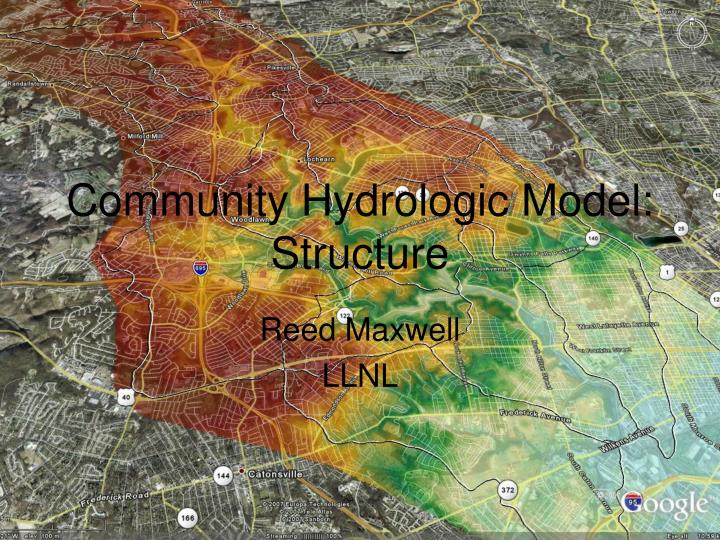
Community Hydrologic Model: Structure. Reed Maxwell LLNL. Challenges to CHM. Application: pore-scale groundwater contaminant transport to global hydrology Physics and scale: balance laws not scale invariant Computing: desktop to supercomputer

E N D
Community Hydrologic Model: Structure Reed Maxwell LLNL
Challenges to CHM • Application: pore-scale groundwater contaminant transport to global hydrology • Physics and scale: balance laws not scale invariant • Computing: desktop to supercomputer • Calibration, Optimization: needs to be flexible to connect w/ management codes • User Communities: each with different needs, goals and perspectives
Huge range in scales Regional Scale: 132x88x0.5km Dx=Dy=1km Dz=0.5m Plot Scale: 17x10x3.8m Dx=Dy=0.34m Dz=0.038m
Timescales and scaling in Groundwater • Range of paths and scales in groundwater • Water moves as K/q~10-4-10-5 m/s • Pressure propagates as Kb/Ss~100-101 m/s • System responds over a wide range of scales (Kirchner et al 2000, 2001; Alley et al 2002) • Topography and land surface processes have strong influence Z (m) Land surface 0 20 40 Travel time (y) Kirchner et al (2000)
Thoughts on Model Structure • Object oriented • Open source • Parallel with efficient solvers, linear scaling • Flexible grid options • Flexible physics options • Flexible input • Not in a vacuum: able to be coupled to other models, processes
Open Source Programming Tools QGIS • an open source and free "Programmable Geographic Information System" • a mapping tool, a GIS modeling system, and a GIS application programming interface (API) all in one • a platform independent Open Source Geographic Information System that runs on Linux, Unix, Mac OSX, and Windows • libraries for raster and vector geospatial formats • Object relational database is handled using PostgreSQL • GRASS compatible Qt/C++ - tools for programming the interface and visualization
ParFlow Structure TCL input script: Set database keys for simulation, any other manipulations. • pfrun command: • Executes parflow.tcl script • Write database (.pfidb) file • Set up parallel run parameters • Execute run script • run script: • Execute ParFlow using platform specific options • Port standard output to a file
Model Input Structure • TCL/TK scripting language • All parameters input as keys using pfset command • Keys used to build a database that ParFlow uses • ParFlow executed by pfrun command • Since input file is a script may be run like a program
SolidFile Geometry (input file) pfset GeomInput.Names "solidinput" pfset GeomInput.solidinput.InputType SolidFile pfset GeomInput.solidinput.GeomNames domain pfset GeomInput.solidinput.FileName fors2_hf.pfsol pfset Geom.domain.Patches "infiltration z-upper x-lower y-lower x-upper y-upper z-lower"
Octree used to delineate geometries Source: Wikipedia
Overland (hillslope rills) and channel flow along 1d links defined from DEM data CATHY Model: Governing equations: channel and hillslope routing [Orlandini & Rosso, WRR 2001]: • "Constant critical support area": overland flow cells with upstream drainage area A < A*; else channel flow • Leopold & Maddock relationships; • Muskingum-Cunge solution scheme (explicit and sequential); etc • (need Pe and Cu1)
Penn State Integrated Hydrologic Model: PIHM Qu and Duffy 2007
ParFlow enables simulating groundwater flow in large subsurface regimes Ground Surface • Two Modes: fully and variably saturated (via Richards’ EQ) flow solver • Efficient multigrid preconditioned linear solver • Kinsol nonlinear solver • Parallel code specifically designed to run on large institutional computer facilities • Enables large, highly-resolved, simulations • Coupled overland flow and land surface interactions Infiltration Front Vadose Zone Saturated Zone Water Table Ashby and Falgout, 1996; Jones and Woodward, 2001; Kollet and Maxwell, 2006
LSM LSM LSM LSM LSM LSM LSM LSM LSM LSM Coupled Model PF.CLM Atmospheric Forcing Land Surface Flow Divide • PF.CLM= Parflow (PF) + Common Land Model (CLM) Kollet and Maxwell (2008), Kollet and Maxwell (2006), Maxwell and Miller (2005), Dai et al. (2003), Jones and Woodward (2001); Ashby and Falgout (1996) • Surface and soil column/root zone hydrology calculated by PF (removed from CLM) • Overland flow/runoff handled by fully-coupled overland flow BC in PF (Kollet and Maxwell, AWR, 2006) • CLM is incorporated into PF as a module- fully coupled, fully mass conservative, fully parallel Air Root Zone Vadose Zone Vegetation Water Table Routed Water Flow Lines Groundwater Dynamically coupled, 2D/3D OF/LS/GW Model
Integration of Atmospheric Processes – PF.ARPS • Understanding two-way feedbacks: subsurface atmosphere • Integrate ARPS (Advanced Regional Prediction System) into ParFlow • ARPS (Xue et al., 1995, 2000, 2001): • Large eddy simulation code • solves the three-dimensional, compressible, non-hydrostatic Navier-Stokes equations • Land Surface Model: ISBA (Interaction Soil Biosphere Atmosphere)
Scaled Parallel Efficiency Perfect efficiency: double problem size and processor # same run time => E = 1 Kollet and Maxwell, AWR (2006)
Many options for subsurface conceptual model Loam Sand • Completely general, 3D subsurface variably saturated GW model • Any parameter combinations, effective, heterogeneous, stochastic • Many scales, features can be incorporated, no predefined GW or vadose zones Loamy Sand Clay Loam Soil Aquifer Aquitard/bedrock
Conceptual Model + GeoDataBase = A Priori Data Conceptual Model Groundwater flow in the Allegheny Plateau Section. Example of the GIS for the surface geology coverage.
Little Washita watershed in OK provides a good field site for coupled model • Site of several Southern Great Plains (SGP) field campaigns • Located at bottom Atmospheric Radiation Measurement (ARM) site • Most complete data set to validate model
“Offline” Model Spinup and Dynamics • Run offline, PF.CLM coupled model • WY 1999 used as forcing (NARR) • Spinup: Run over successive years until beginning-ending water and energy balances drop below threshold • Results can be: • compared to data • used to understand dynamics • used for initialization Kollet and Maxwell (2008a)
Water Table Depth, Cross Section • Water table driven by topography • Very deep (~40m) at hilltops (drier) • Very shallow in valleys (wetter) • Cross section shows variation of WT and Saturation hilltops valleys groundwater Maxwell, Chow and Kollet, AWR (2007)
We see a connection between groundwater and the lower atmosphere 27h • Cross-section at y=15km • Shallow WT=wetter • Wetter=cooler • Temperature variations=wind variations • Wind variations=BL variations Maxwell, Chow and Kollet, AWR (2007)
Vegetation effect: 15 Wm-2 Groundwater effect: 25 Wm-2 Influence of Groundwater Dynamics on Energy Fluxes (yearly averaged) Kollet and Maxwell (2008a)
Understanding Residence Times: Spatiotemporal Scaling of Baseflow Contributions Kollet and Maxwell (2008b)
Summary: CHyMP Model Structure • Object oriented • Flexible • Range of interface, data, needs • Range of Scales • Growing community of models, experiences • Interesting science questions
CHyMP Model Challenges • Community • Intercomparison • Education • Data