Electron Collimator Design for the Little “a” Measurement

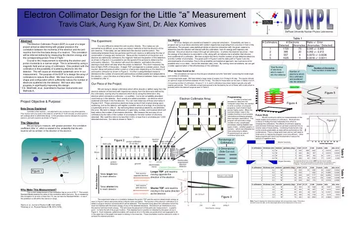
1. Figure 4 Electron Path Electron Collimators Longer TOF: anti-neutrino moving opposite the direction of the electron Shorter TOF: anti-neutrino moving in the same direction as the electron Figure 5 Figure 3 Anti-neutrino Direction of Anti-Neutrino Neutron Proton Renderings of Collimators Direction of Electron θ 2-Dimensional (Side Cut-out) 3-Dimensional Figure 1 Electron Electron Direction Anti-neutrino (with electron) θ Electron Collimator Design for the Little “a” Measurement Travis Clark, Aung Kyaw Sint, Dr. Alex Komives DUNPL DePauw University Nuclear Physics Laboratories Table 1 Our Method All of our designs are created and tested in computer simulation. Essentially, we have a program set up to produce electrons with random trajectories originating from a source in front of the collimators. The program uses statistical tables on electron interaction with the given material to determine how the electron will interact with the collimators: how it’s energy and trajectory are affected. Should an electron make it through all collimators – to where the detector would be – then the energy of that electron is recorded in a file, along with an indicator as to whether that electron ever scattered off a collimator. We then analyze this file to find the number of total detected electrons and the number of anomalies. The green path in Figure 4 and the dark path in Figure 5 are the simulated paths of anomalies. Due to this probability and statistical approach, we must account for possible error in our data – hence the absolute (abs.) error. By running more simulations, we can get a better approximation of the effectiveness of the collimator. What we have found so far The simulations we have run thus far give indications as to the “best bets” concerning the inside angle and number of collimators. Concerning inside angle. We have tested a large range of angles, from 30 deg to 80 deg. The results indicate an optimum angle somewhere between 45 and 70 deg. The data for these tests can be seen in Tables 3 and 4. Concerning number of collimators. Arrays of 1, 2, 3, and 5 collimators have been tested, typically only with washer geometries. The 5 collimator arrays have proved to be the best by far out of these, with a ratio which is probably within the desired range as seen in Table 2. Abstract The Electron Collimator Project (ECP) is a part of a larger project aimed at determining with greater precision the correlation between the momenta of the electron and the anti-neutrino from the free beta decay of a neutron. This correlation will be inferred indirectly by measuring the electron energy and the corresponding proton Time of Flight.1 Crucial to this measurement is restricting the electron and proton momenta to a narrow range. This is achieved by using a magnetic field and an array of collimators. One problem with the collimators is the possibility of scattering electrons into the detector. This will cause an intolerable systematic error in our measurement. The purpose of the ECP is to design the array of collimators to reduce this effect. We have found a collimator shape and configuration which sufficiently reduce the number of electrons scattered into the detector. We have also made progress in significantly improving this design. 1 F.E. WeitFeldt, et.al., Submitted to Nuclear Instruments and Methods A. The Experiment: It is very difficult to detect the anti-neutrino directly. This makes our job somewhat more difficult, as we must use indirect methods to find the direction of the anti-neutrino. Fortunately, we can detect both the electron and the proton. The relationship between these two particles and the anti-neutrino is defined by the law of conservation of energy and momentum. Because the momentum of the proton and electron are defined by collimators, the magnetic field and the position of the detectors as shown in Figure 2, it is possible to use the speed of the protons to determine the antineutrino direction. The electron will reach the detector, well before the proton, starting a clock which will stop when the proton is detected. This clock measures the time-of-flight (TOF) of the proton. A larger TOF corresponds to a slower proton. Each neutron decay will produce either a slow or a fast proton depending on the direction of antineutrino emission as shown in Figure 3. It is then a straightforward matter to deteremine the number of events with antineutrinos emitted parallel and antiparallel to the electron – count the slow and fast protons. The difference between these numbers is related to Little “a”. Our Piece of the Project: We are trying to design collimators which either absorb or deflect away from the electron detector all electrons with trajectories varying from the dimension defined by the collimators, leaving only the electrons which do lie along that dimension. Any electron which intersects a collimator – or scatters – but is not completely absorbed could end up in the detector. Such events are called anomalies – an electron which scattered and made it into the detector. You can view instances of these anomalies in Figures 4 & 5. These anomalous electrons loose some of their original energy upon scattering, and so the detector will register a smaller amount of energy, thus producing a systematic error in Little “a”. By removing these anomalous electrons, we eliminate this error. We wish to design collimators of a geometry, number, and material which will best reduce the number of anomalous electrons. We measure the accuracy of our collimators by the ratio of the number of anomalies to the total number of electrons detected. We need this ratio to be less than 0.003, or less than 3 anomalies per 1,000 detected electrons. Our data is shown in Table 1. Ratio= Total Number of electrons which made it into the detector Number of Anomalies Total number of detections Number of electrons which hit a collimator and scattered into the detector Programming In order to extract and process our data from the computer output files, we needed to write a number of computer programs, most of which have proven highly useful. When the summer ended, I was in the middle of writing a much smarter information processing program than had been used before. This program will automate a large number of very complicated processes, making feasible new types of data – whether graphic or numeric – which are otherwise too time-consuming to obtain. Programming is an area of extensive future work. Electron Collimator Array Project Objective & Purpose: Beta Decay Explained Consider a free neutron – not adjoined to any nucleus or any other particle. This neutron will only exist in this state for a half-life of 10.24 minutes, at which point it will undergo what is called beta decay. In this process a neutron decays into a proton, electron, and anti-neutrino as shown in Figure 1. The Objective We are trying to measure, with greater precision, the correlation coefficient, little “a”, which is related to the probability that the anti-neutrino will be emitted in the direction of the electron. Why Make This Measurement? The current measurement of this correlation has an error of 4%.2,3 The current Standard Model predicts the value of this correlation within that error. By re-measuring this correlation to an error of less than 1%, we can test the Standard Model – to see if the prediction is still within the new error range. 2Byrne et. al., Journal of Physics G 28, 1325 (2002). 3Stratowa et. al., Physical Review D 18, 3970 (1978). Electrons Future Work We will continue to refine our measurements on the inside angles and numbers of collimators. Work will also continue in finding the best material(s) from which to compose the collimators. The effects of collimator spacing and collimator thickness have not yet been examined; this is another area of future testing. Combining these factors may not be entirely predictable, so tests will be performed on the combinations. This is a large work-load, and so I will need to finish work on making the program more time-efficient. Other large programs will need to be finished which reduce the amount of repetitive work. Electron Detector Figure 6 Figure 2 Washer Geometry Table 2 Angled Geometry The angle described in this column (OMIT: the chart columns entitled “geometry”) is the off-vertical angle of the inside face of the collimators, given in degrees. This angle is shown in the figure to the left, represented by θ. Table 3 Anti-neutrino (opposite electron) Takes longer time to reach detector Takes shorter time to reach detector proton momentum Proton Detector Table 4 proton momentum The experiment relies on a correlation between the proton TOF and the electron (beta) kinetic energy as seen in Figure 3 which was produced by a Monte Carlo simulation. The function of the electron collimators is to select a range of electron momenta which will be detected. The important thing about the collimators is that they must not interfere with the kinetic energy of any of the detected electrons. Should such an interference occur, the electron will lose kinetic energy. This will cause the placement of that particular measurement – a graphic point – to fall to the left of its proper location. This displacement in position is indicated by the green arrow in Figure 3. Such instances, called anomalies, will cause an error in the data, as points which are supposed to lie in the upper bar of the graph now seem to belong in the lower bar. These anomalies must be reduced in order to achieve the desired precision. Note: Figure 6 displays the relationship between ratio and geometry angle. Remember, we want a very low ratio, so the ideal angle will be at the lowest point on the curve.