Download
1 / 32
320 likes | 440 Views
Hierarchical Modeling for Economic Analysis of Biological Systems: Value and Risk of Insecticide Applications for Corn Borer Control in Sweet Corn Economics and Risk of Sweet Corn IPM. Paul D. Mitchell Agricultural and Applied Economics University of Wisconsin-Madison

E N D
Hierarchical Modeling for Economic Analysis of Biological Systems: Value and Risk of Insecticide Applications for Corn Borer Control in Sweet CornEconomics and Risk of Sweet Corn IPM Paul D. Mitchell Agricultural and Applied Economics University of Wisconsin-Madison University of Minnesota Department of Entomology Seminar April 11, 2006
Goal Today 1) Explain and illustrate Hierarchical Modeling 2) Provide economic intuition of findings concerning the economic value of IPM for sweet corn • Overview work in progress with Bill Hutchison and Terry Hurley on sweet corn IPM as part of a NC-IPM grant • All work in progress
Problem/Issue • Use existing insecticide field trial data to estimate the value and risk of IPM for insecticide based control of European corn borer (ECB) in processing and fresh market sweet corn • Operationally: Do I need another spray? Estimate the expected value of an additional insecticide application for ECB control • Use hierarchical modeling to incorporate risk into the analysis
Conceptual Model • Keep key variables random to capture the risk (uncertainty) in pest control • Develop a hierarchical model = linked conditional probability densities • Estimate pdf of a variable with parameters that depend (are conditional) on variables from another pdf, with parameters that are conditional on variables from another pdf, etc. … … … …
Random Initial ECB Observe ECB Apply Insecticide? Random % Survival gives Random Remaining ECB Random % Marketable Random Pest-Free Yield Random Price Net Returns Net Returns = P x Y x %Mkt – Pi x AIi – #Sprys x CostApp – COP
Random Initial ECB • Mitchell et al. (2002): 2nd generation ECB larval population density per plant collected by state agencies in MN, WI, IL • Empirically support lognormal density with no autocorrelation (new draw each year) • Sweet corn has more ECB pressure, so use MN & WI insecticide trial data for mean and st. dev., pooling over years 1990-2003 • Lognormal density: mean = 1.28, CV = 78%
Insecticide Efficacy Data • Efficacy data from pyrethroid trials (~ 50) • Capture, Warrior, Baythroid, Mustang, Pounce • Most data from: MN, WI, IN and ESA’s AMT • Data include: • Mean ECB larvae/ear for treated and untreated (control) plots of sweet corn • Percentage yield marketable for processing and for fresh market • Number of sprays and application rate
Random ECB after Sprays • Model: ECB = ECB0 x (% Survival)sprays • Example: ECB0 = 4, 50% survival per spray, 2 sprays, then ECB = 4(½)2 = 1 • Rearrange: % Survival = (ECB/ECB0)1/sprays • Geometric mean of % Survival per spray • Use observed ECB, ECB0, and number of sprays to construct dependent variable: “Average % survival per spray”
Random % Survival • Dependent variable: Average % Survival per spray • Regressors • ECB0 (density dependence) • Number sprays (decreasing returns) • Chemical specific effect • Beta density (0 to 1) with separate equations for mean and st. dev. (Mitchell et al. 2004) • Mean = exp(b0 + b1ECB0 + b2Sprays + aiRatei) • St. Dev. = exp(s0 + s1Sprays)
Model Implications • Mean = exp(b0 + b1ECB0 + b2Sprays + aiRatei) • ECB0 increase: Mean %S decreases since b1 < 0 • Density dependence: more ECB, lower survival rate • Ratei increase: Mean %S decreases since ai < 0 • More insecticide, lower survival rate • Use a’s to compare across insecticides • Warrior>Capture>Baythroid>Mustang>Pounce • Spray increase: Mean %S increases since b2 > 0 • Average survival rate per spray increases with sprays • Total survival rate = %Surivialsprays decreases
Illustration of average %S per spray and total %S with Capture at a rate of 0.04 AI/ac with ECB0 of 2
Effect of ECB0 on conditional pdf of avg %Survival per spray RED: ECB0 = 1GREEN: ECB0 = 3BLUE: ECB0 = 5 Randomly drawn ECB0 affects % Survival pdf
Effect of sprays on conditional pdf of avg %Survival per spray RED: 1 sprayGREEN: 3 spraysBLUE: 5 sprays Chosen number of sprays affects % Survival pdf
Hierarchical Model Series of Linked Conditional pdf’s • Draw Random ECB0 from lognormal • Draw Average % Survival per spray from beta with mean and st. dev. depending on ECB0, number of sprays, chemical, and rate • Calculate ECB = ECB0 x (% Survival)sprays • Draw % Marketable depending on ECB • Draw yield and price, calculate net returns • Unconditional pdf for ECB or net returns = ??? • Must Monte Carlo simulate and use histograms and characterize pdf with mean, st. dev., etc.
lognormal density Random Initial ECB Observe ECB Apply Insecticide? Random % Survival gives Random Remaining ECB transformed beta times lognormal beta densities Random % Marketable Random Pest-Free Yield Random Price Net Returns lognormal density Net Returns = P x Y x %Mkt – Pi x AIi – #Sprys x CostApp – COP
Rest of the Model: Quick Summary • % Marketable for Processing or Fresh Market has beta density (0 to 1) • mean = exp(k0 + k1ECB), constant st. dev. • More ECB, on average lower percentage marketable (exponential decrease) • Pest Free yield has beta density (common) • Minimum: 0 tons/ac • Maximum: 9.9 tons/ac (mean + 2 st. dev.) • Mean: 6.6 tons/ac (WI NASS 3-yr avg.) • CV: 25% (increase WI NASS state CV)
Prices and Costs • Sweet Corn: $67.60/ton • Insecticides ($/ac-treatment) • Capture Warrior Baythroid $2.82/ac $3.49/ac $6.09/ac • Mustang Pounce $2.80/ac $3.76/ac • Aerial Application: $4.85/ac-treatment • Other Costs of Production: $200/ac • No Cost for ECB Scouting, Farmer Management Time, or Land
Value of 1st spray: $115-125/ac • 1 Scheduled Spray and use of IPM for 2nd spray maximizes farmer returns
Economic Thresholds (ECB larvae/ear) 2nd spray: 0.15 3rd spray: 0.20 4th spray: 0.25
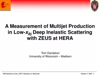
IPM has lower risk (lower standard deviation) than scheduled sprays
Source of IPM value is preventing unneeded sprays • IPM more value for Baythroid and Warrior, since cost more • IPM more value after more sprays, since need fewer sprays
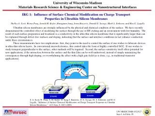
With proportional yield loss from pest, pests usually reduce st. dev. of returns, so pest control increases st. dev. of returns • IPM decreases st. dev. of returns since more pests • More sprays increases st. dev. of returns since fewer pests
Caveats • Can’t do “Sequential” IPM: observe and decide multiple times during season • Data only allow estimation of average % survival per spay for many sprays • Need different data for “true” IPM • Current data readily available easy to collect while required data are expensive to obtain • Canning companies control sprays and they are not necessarily maximizing farmer returns
Processing versus Fresh Market • IPM for Processing sweet corn • 1 scheduled spray and use of IPM for the 2nd spray maximizes farmer returns • First scheduled spray worth $115-$125/ac • IPM increases mean returns $5-$10/ac (~ one spray), not including scouting costs • IPM decreases st. dev. of returns slightly • Similar analysis for Fresh Market sweet corn • IPM decreases mean returns • IPM decreases st. dev. of returns
Fresh Market Sweet Corn • Same basic model structure with updates • Pest free yield: 1100 doz/ac with 25% CV • Price: $2.75/doz with st. dev of $0.60/doz • % marketable for fresh market • mean = exp(k0 + k1ECB), constant st. dev. • Six scheduled sprays maximize returns • Optimal IPM threshold = zero
Benefit vs. Cost of IPM • Benefit of IPM: Preventing unneeded sprays • Cost of IPM: Missing needed sprays, plus cost of information collection • More valuable crop makes missing needed sprays too costly relative to low cost insecticides • Few will risk $1000/ac to try saving $10/ac • “Penny Wise-Pound Foolish”
Economic Injury Level • Pedigo’s Classic EIL = C/(V x I x D x K) • EIL = pest density that causes damage that it would be economical to control • C = cost of control • V = value of crop • I x D = injury per pest x damage per injury • K = % Kill of pest by control • As V becomes large relative to C, the EIL goes to zero
Fresh Market Sweet Corn IPM • Insecticide too cheap relative to value of fresh market sweet corn to make IPM valuable • Insect pests vs insect terrorists (IPM or ITM?) • Insecticide cost must increase so IPM creates more value by preventing unneeded sprays • Market prices increase • Environmental costs of insecticide use • Alternatively: more competitive market for pesticide-free or organic sweet corn
Conclusion • Illustrated hierarchical modeling • Capture effect of production practices on risk • Generally requires Monte Carlo simulations • Applied to ECB in sweet corn • Also for ECB and corn rootworm in field corn • IPM for commodity vs. high value crops • If crop becomes too valuable relative to the cost of insecticide, IPM not economical • Processing versus Fresh Market Sweet Corn