Download
1 / 59
680 likes | 1.21k Views
Fault Detection and Diagnosis. Outline. Fault management functionality Event correlations concept Techniques. Definitions. A fault may cause hundreds of alarms. We need to be able to do the following: Detect the existence of faults Locate faults An alarm

E N D
Outline • Fault management functionality • Event correlations concept • Techniques
Definitions • A fault may cause hundreds of alarms. • We need to be able to do the following: • Detect the existence of faults • Locate faults • An alarm • External manifestations of faults • Generated by components • Observable, e.g. via messages • An alarm represents a symptom of a fault. • An event • An occurrence of interest, e.g. an alarm message
Fault Management Functionalities • Fault detection • Should be real-time • Techniques can be based on active schemes (e.g., polling) or event-based schemes (where a system component says that it has detected a failure). • Fault location • Is it a link or system component or application component? • Determine corrective actions • Carry out corrective actions and determine effectiveness
Alarm (Event) Correlation • Alarm explosion • A single problem might trigger multiple symptoms (e.g., router is down) • There could be too many alarms for an administrator to handle; Techniques used to help: • Compression: reduction of multiple occurrences of an alarm into a single alarm • Count: replacement of a number of occurrences of alarms with a new alarm • Suppression: inhibiting a low-priority alarm in the presence of a higher priority alarm • Boolean: substitution of a set of alarms satisfying a condition with a new alarm
Fault Diagnosis • Major application of alarm correlation is fault diagnosis • Useful in fault location
Faults and Alarms • The previous figure shows that correlation c1 detects the fault f1 and that correlation c2 detects the fault f2. • Correlating c1 and c2 into the correlation c0 allows the diagnosis of the fault f0.
Example • Let a1, a2, a3, a4, a5 be alarms generated by client processes indicating that a client process is not getting a response from a server. • Correlation techniques can be used to show that since a1, a2, a3 were generated by client processes by trying to contact the same server then the server may be the problem. Similar comments apply to a4 and a5.
Example • From the perspective of client processes, the servers (at the second level of the previous figure) are at fault. • However, it may be observed that alarms were generated by these two servers. Both alarms indicate that each of the two servers are not getting a response and that both were trying to contact the same server. This is another correlation.
Rule-Based Reasoning • Based on expert systems • Intended to represent heuristic knowledge as rules. • Components • Knowledge Base (KB): Contains the expert rules that describe the action to be taken when a specific condition occurs e.g., if-then-else • Working Memory(WM): Stores information such as the system/network topology and data collected through the monitoring of application and network components.
Rule-Based Reasoning • Components (continued) • Inference engine: matches the current state (as represented by the monitored data) of the system against the left-side of a rule in the knowledge base in order to trigger the action. • The rules are meant to encapsulate expert knowledge • Why rule-based reasoning? • Rules are interpreted which means that rules can be changed without recompiling. • Since expert knowledge can be wrong and/or complete, this feature is very useful.
Approaches • Model-based • Fault propagation • Model traversing • Case-based reasoning
Model-Based Reasoning • Use structural knowledge, e.g., via object-oriented models • To illustrate model-based reasoning, we will look at network equipment. • A network equipment class is used to describe a network equipment type. • Network equipment classes are organized into a hierarchy using class/subclass relations.
Model-Based Reasoning • The root class is a generic class that represents the most general information common to all network equipment e.g., vendor name • The next level of the hierarchy describes the basic network equipment classes such as physical-trunk class and switch class. • Example: The trunk class refers to T1 trunk class and T3 trunk class. • An association class represents a relationship between two object classes that represents connectivity.
Model-Based Reasoning • The network configuration model is constructed from the instances of individual network equipment. • The network configuration model is a graph consisting of objects instantiated from the network equipment classes. If there is an edge between two objects then this implies that the two objects are connected.
Example Csd_syslab router MC Csd_res hub Stats BGS WSC fiber hub Genetics Geophys zoo 10Base-T Fiber optic
Example • There is a Network Equipment class that has attributes used to describe a network equipment. At a minimum assume that there is an attribute representing the name of the vendor. • You can subclass the following from the Network Equipment class: • Connector • Cable Segment
Example • The Connector class has two subclasses: • Hub • Router • The Cable Segment class also has two subclasses: • 10Base-T • Fiber Optic • The Hub class has two subclasses: • Fiber Hub • Local Hub
Network Equipment Cable Segment Connector Hub Router 10Base-T Fiber Hub Fiber Optic Local Hub Example
Model-Based Reasoning • Message Class Hierarchy • Describes messages created by elements of a network configuration model. • These messages report symptoms. They are essentially alarms.
Example • A hub can generate a message stating that one of its ports is “bad”. In fact, there is a message associated with each port. • A hub can generate a message stating that the cable segment on a particular port does not seem to be functioning. This can be encapsulated in a message class called Hub_Report_Port_Bad. This can be subclassed into messages generated by each type of hub.
Model-Based Reasoning • Correlations • Conditions under which the correlations are asserted • Correlations are stated in terms of message classes. • At run-time there is match between an instantiation and a message class. • Example: If a local hub is connected to more than one router and there are two messages from the routers indicating that there are problems connecting to the local hub then this is a good indication that the hub is a problem.
Fault Propagation • Based on models that describe which symptoms will be observed if a specific fault occurs. • Monitors typically collect managed data at network elements and detect out of tolerance conditions, generating appropriate alarms. • An event model is used by a management application to analyze these alarms. • The event model represents knowledge of events and their causal relationships.
Fault Propogation (Coding Approach) • Correlation is concerned with analysis of causal relations among events. • The notation ef is to denote causality of the event f by the event e. • Causality is a partial order between events. • The relation may be described by a causality graph whose directed edges represent causality. • Distinguish between fault events (faults or problems) and symptom events (symptoms). • Nodes of a causality graph may be marked as problems (P) or symptoms (S). • Some symptoms are not directly caused by faults, but rather by other symptoms.
Fault Propagation (Coding Approach) Example Causality Graph 11 10 9 5 8 7 6 3 4 1 2
Fault Propagation (Coding Approach) • The correlation problem • A correlation p s means that problem p can cause a chain of events leading to the symptom s. • This can be represented by a graph.
Fault Propagation (Coding Approach) A Correlation Graph 9 10 6 11 1 2
Fault Propagation (Coding Approach) • For each fault (problem) p, the correlation graphs provides a vector that summarizes information available about correlation and symptoms and problems. • This is referred to as the code of the problem. • Alarms may also be described using a vector assigning measures of 1 and 0 to observed and unobserved symptoms. • The alarm correlation problem is that of finding problems whose codes optimally match an observed alarm vector.
Fault Propagation (Coding Approach) • Example codes (look at correlation graph example) • 1 = (0,1,1) – This indicates that problem 1 causes symptoms 9 and 10 • 2 = (1,0,1) – This indicates that problem 2 causes symptoms 6 and 10 • 11 = (0,1,1) – This indicates that problem 11 causes symptoms 9 and 10.
Fault Propagation (Coding Approach) • Example alarm vector • Assume that alarms indicating symptoms 3 and 9 have been observed. • a = (0,1,1) • We can infer that either 1 or 11 match the observation a. • These two problems have identical codes and hence are indistinguishable. • The fault management application may have to do additional tests.
Fault Propagation (Coding Approach) • A Codebook is an array of the vectors just defined. • The number of symptoms associated with a single problem may be very large. • Sometimes a much smaller set of symptoms is selected to accomplish a desired level of distinction among problems.
Fault Propagation (Coding Approach) Example Codebook p1 p2 p3 p4 p5 p6 1 1 0 0 1 0 1 2 1 1 1 1 0 0 4 1 0 1 0 1 0
Fault Propagation (Coding Approach) Example Codebook p1 p2 p3 p4 p5 p6 1 1 0 0 1 0 1 3 1 1 0 1 0 0 4 1 0 1 0 1 0 6 1 1 1 0 0 1 9 0 1 0 0 1 1 18 0 1 1 1 0 0
Fault Propagation (Coding Approach) • Distinction among problems is measured by the Hamming Distance between their codes • The radius of a codebook is one half of the minimal Hamming distance among codes. • When the radius is 0.5, the code provides distinction between problems.
Fault Propagation (Coding Approach) • Is this easy to apply to application processes? • No • Why • Applications are dynamic • The coding approach assumes the system is fairly static.
Model Traversing • Reconstruct fault propagation at run time using relationships between objects • Begins with managed object that generated event • Work best when object relationship is graph-like and easy to obtain since it must be obtained at run-time • Performance • Potential parallelism • Weaknesses • Lack of flexibility • Not well-structured like fault propagation
Model Traversing • Characteristics • Event-Driven: Fault management application is passive until an event arrives. This event is the reporting of a symptom. • Correlation : Decides whether two events result from the same primary fault. • Relationship Exploration: The fault management application correlates events by detecting special relationships between the source objects of those events.
Model Traversing • Event reports should have the following information: • Symptom type • Source • Target • etc • If symptom si’s target is the same as sj’s source then this is an indication that si is a secondary symptom. This allows us to ignore certain alarms.
Model Traversing • For each event, construct a graph of objects (models) related to the source object of that event. • When two such graphs touch each other, i.e. contain at least one common object, the events which initiated their construction are regarded to be correlated. Possibly these two events are the result of the same fault. • If si is correlated with sj and sj is correlated with sk then through transitivity we can conclude that si is a secondary symptom.
Model Traversing • The process of eliminating symptom reports may result in reports that have the same target. • Example: • s1 and t • s2 and t • It might be necessary to construct possible paths of objects between s1 and t as well as s2 and t • Nodes in common are good candidates for the faults.
Model Traversing • We will now discuss the building of graphs • The algorithm for building graphs uses relationships between network hardware and software components to search for the root cause of a problem. • Assumes that information about the relationships between the components are available (e.g., through a database). • Assumes that there are functions including these: • getNextHop(source, target,B): Get the node representing the next entity (that comes after B) in the path between source and target. Note that this may return more than one entity.
Model Traversing Example • Assume the following configuration of processes and machines. All machines are connected through the Ethernet. • P1 is on chocolate; P2 is on peppermint • P3 is on vanilla; P4 is on strawberry • P5 is on doublefudge; P6 is on mintchip • Communication is through remote procedure calls. This basically requires that all communication go through a daemon process on the server host’s machine. We will call this rpcd
P6 P2 P5 P3 P1 P4 Model Traversing Call structure is depicted in the following graph:
Model Traversing Example • Assume that P4 terminates abnormally causing a cascade of timeouts • Correlation will result on focusing on these event reports: • (P1,P4) • (P3,P4) • Not enough to diagnose the fault. • It’s all at the process level. • There are still many entities or objects to examine since you do not want everything generating a message.
Model Traversing • Example • Starting with P1 the next component (node) along the path of the connection between P1 and P4 is identified. • Between P1 and P4 are many entities. We will start out with a vertical search which basically results in the fact that P1 is running on a host machine called chocolate
Model Traversing • chocolate is connected to the hub through an ethernet cable. • The hub is connected to strawberry through an ethernet connection cable where P2 is running. Thus we can say that the path is the following: • P1, chocolate,ethernet connection cable,hub,strawberry,ethernet connection cable, rpcd.strawberry,P4 • The path between P3 and P4 is the following: • P3, vanilla, ethernet connection cable, hub, ethernet connection cable, strawberry, rpcd.strawberry, P4
Model Traversing Example • This suggests that we can narrow down the problem to hub, ethernet connection cable, strawberry.rpcd, strawberry, P4. • At this point, the fault management application may want to poll for additional information. The polling may check to see if something is up or not. An example is applying the ping operation to the host machine called strawberry. • What if every entity is up? This may indicate that strawberry is overloaded. An indication of an overload can be found by measuring the CPU load.
Model Traversing • Building the graphs requires structural information and the use of rules.
Model Traversing Implementation • What management services are needed? • To detect and report symptoms, one could use application instrumentation. • The instrumentation library should most likely talk with a management process (or agent). • The agent sends an event report to the event server. • The event server may have a set of rules for symptom correlation. • After correlation, a task may be invoked that does relationship exploration and the final diagnosis.