Download
1 / 45
450 likes | 594 Views
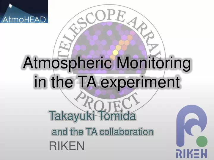
Atmospheric Monitoring in the TA experiment. Takayuki Tomida and the TA collaboration RIKEN. Telescope Array(TA ) Experiment. Hybrid observation : SD (507 units) + FD (3 locations: 38 units). Fluorescence Detector (FD ). Surface Detectors SDs Plastic scintillator.

E N D
Atmospheric Monitoringin the TA experiment Takayuki Tomida and the TA collaboration RIKEN
Telescope Array(TA) Experiment Hybrid observation: SD (507 units) + FD (3 locations: 38 units) Fluorescence Detector (FD) Surface Detectors SDs Plastic scintillator The joint experiment with Japan, the United States , South Korea, Belugiumand Russia. The observation started in Apr. 2008 North American at Utah
Atmospheric monitor in TA • LIDAR • CLF • LIDAR@CLF • IR camera • CCD camera • weather monitor LR
Contents • LIDAR observation The atmospheric transparency model of two kinds of altitude distribution was determined. • Influence of using LIDAR’satmospheric transparency for FD reconstruction. FD reconstruct fluctuation was estimated by using the atmospheric model. • CLF Observation Correlated to the time variationswas observed when compared to the CLF and LIDAR by Optical Depth. • IR camera Observation • Eye-scan
LIDAR System LIDAR BRM-St. 100m Telescope & dome of TA LIDAR BRM Station Measurement : Before and After FD observation Datacondition for determination atmospheric model
Models of Atmospheric transparency 1σ=+83%/-36%. single exponential double exponential Extinction coefficient at each height VAOD at each height Double exponential Model Single exponential Model
Seasonally Aerosol scattering summer winter Median of VAOD for different seasons Distribution of VAOD at 5km above ground level for different seasons +0.020 - 0.012 Summer: 0.039 The effect of the aerosol component in summer is 1.5 times greater than that inwinter. +0.010 - 0.007 Winter : 0.025
Fluctuation of FD reconstruction using atmospheric transparency by the LIDAR measurement. =Method= • MC simulation using daily atmospheric transparency to create a shower data. • Simulated data are reconstructed using daily atmospheric transparency or model function. • Estimating the impact of using a model function to compare the results with the reconstruction of each atmospheric transparency. • ΔE is evaluated by the ratio, ΔXMax will be evaluated by difference. • Reconstruction using Daily atmospheric data or two atmospheric models =Simulation conditions= • Primary energy : logE= 18.5, 19.0 and 19.5 eV • Direction: Zenith is between 0 ∼ 60 ◦ (the isotropic) Azimuth is between 0 ∼ 360 ◦ (the isotropic) • Core position : within 25 km of the CLF (center of TA FDs). • Number of event : 20 events at each energy for each of 136 good LIDAR runs. • Quality Cuts : Reconstructed Xmax in field of view of FD.
Fluctuations by using the atmospheric model Daily vs model func. @logE=19.5 eV XMax Energy Comparison of reconstructed fluctuation in atmospheric model. The fluctuation not containing the reconstruction bias using atmospheric model at each energy Rec. ΔE: 6%@18.5 9%@19.0 11%@19.5 Rec. ΔXmax : 9g@18.5 9g@19.0 9g@19.5
CLF System Starting CLF operation :2008.Dec〜 CLF container and power generation system and optics of CLF Optical diagram of the CLF CLF laser is injected into FD’s FOV :300 shots :10Hz :vertical direction :every 30 minutes. Block diagram of devices for CLF
CLF‘s observation image VAOD eq.
analysis method Uniform atmospheric No aerosols
VAOD (Example) & Comparison of BR &LR VAOD (LR) VAOD (BR)
Conclusion of LIDAR • The extinctioncoefficient α is obtained from LIDAR observation, then the VAOD τAS(h) is defined as the integration of α from the ground to height h. • A model of αAS with altitude was found by fitting two years of LIDAR observations. • The range of variation of the daily data from the model is +83%/-36%. • When 1019.5 eV air shower is reconstructed using the model function, the systematic uncertainty of energy is shown to be about 11%. • And the systematic uncertainty of XMax to be about 9 g/cm2 by comparing MC simulation data.
Conclusion of CLF • VAOD was analyzed by using the CLF event of high view camera's. • BR and LR are consistent with a few %. • There is a correlation VAOD measured in each of the CLF and LIDAR. • Using the CLF, will be able to interpolate for the atmospheric transparency of the period where have not been observed by LIDAR.
Hardware (general drawing) • Back-scatter detector is set up on top of the CLF. • LIDAR@CLF use PMT of 20mm and 38mm in diameter. • telescope & 20mm PMT for High altitude (1.5~7.0~ km) • 38mm PMT for Low altitude (~2.5km) LIDAR@CLF system Fig. Block diagram of LIDAR@CLF Fig. general drawing of LIDAR@CLF
Sensitive 8 ~ 14 us • 320 x 236 pixels • FOV: 25.8ox 19.5o • Near the LIDAR dome • Once every 50 min (~2009Jul) • or 30min (2009Jul~) TA IR camera 236, 19.5o 320, 25.8o 7 8 9 10 11 12 6 5 4 3 1 2
Clear IR Sky Images If there are clouds, the sky looks warmer. An IR image are split into 4 “sections” horizontally in data analysis, because lower elevation region looks like warmer. Deciding the probability of cloud in each section and each season. sec1 sec2 sec3 sec4 Cloudy sec1 sec2 sec3 sec4 D: Pixel Data
p=0.05 p=0.21 Score = 2.18/4.00 Examples p=0.92 p=1.00 Total: 1.05/48.0 Clear night Total: 47.0/48.0 Cloudy night Total: 13.0/48.0 0.034 0.035 0.029 1.991 3.790 0.174 Sparse night 0.068 0.653 1.314 1.532 2.046 3.834
IR Camera Score Sum of Scores of All the Directions • Sections 3&4 of Bottom layer exclude from analysis. • The ratio of clear-cloudy nights is about 7 to 3. Cloudy Clear
Eye’s scan Code IR Camera Score Comparison between IR and Eye-scan • Eye’s-Scan Code is index of the cloud to determine in the observer's eye to the FD observation night. • The code is a total of 6 points. • IR score and Eye-scan code is consistent. Cloudy Clear
Comparison between IR and CLF • The data is extracted, when CLF and IR operate within 10 minutes • Color-coded a histogram of the IR score by CLF’s weather condition. • IR score and CLF data is consistent. Examples are determined to cloudy in CLF
Conclusions (Cloud monitor) • About 70% of the TA observation night is Clear night • IR score and Eye-scan code is consistent. • IR score and CLF data is consistent.
Typicals of Extinction Coefficient Aerosol distributed only low height less Aerosol scattering α 10 Height above ground [km] Aerosol distributed high height Aerosol distributed both height
Typicals of VAOD Aerosol distributed only low height less Aerosol scattering VAOD 10 Height above ground [km] Aerosol distributed high height Aerosol distributed both height
Comparison between BR and LR(2009.08.26〜2010.02.14) • VAOD of LR is larger than 6% more BR. • The adjustment of de-polarization was shifted slightly • in this observation term. • The likely influence of de-polarization adjustment. • For future, I will confirm in another observation term.
Comparison between LIDAR and CLF • Conditions • 2009.Sep〜2009.Dec • No cloud • |Timelidar-TimeCLF| <1hr
Effects on energyby atmospheric fluctuation single component 18.5 19.0 19.5 double component 18.5 19.0 19.5
VAOD (LR) VAOD (BR)
Effects on Xmaxby atmospheric fluctuation single component 18.5 19.0 19.5 double component 18.5 19.0 19.5
Fluctuation of reconstruction by each atmospheric logE=19.5 eV XMax Energy The fluctuation Including the reconstruction bias using atmospheric model at each energy are result of reconstruction by each atmospheric conditions. Rec. ΔE: 10%@18.5 12%@19.0 16%@19.5 Rec. ΔXmax : 19g@18.5 18g@19.0 10g@19.5
Rayleigh scattering Jan Apr Jul Nov
Date variation of VAOD@8km & 10km • Winter atmosphere may be clear. • There is correlation with LIDAR.
Analysis policy of LIDAR@CLF Analytical result only of LIDAR@CLF Analytical result only of CLF ? × × ? + VAOD VAOD Height[km] Height[km] Normalized by VAOD of CLF. • Shape of VAOD according to height is determined from LIDAR@CLF. • VAOD at high altitude is determined from the analysis of CLF. × × VAOD Analytical result of LIDAR@CLF and CLF 42
Fluctuation of FD reconstruction using atmospheric transparencyby the LIDAR measurement.
Typicals of Extinction Coefficient Aerosol distributed only low height less Aerosol scattering α α 0 5 10 Height above ground [km] 0 5 10 Height above ground [km] Aerosol distributed high height Aerosol distributed both height α α 0 5 10 Height above ground [km] 0 5 10 Height above ground [km]
Typicals of VAOD Aerosol distributed only low height less Aerosol scattering VAOD VAOD 0 5 10 Height above ground [km] 0 5 10 Height above ground [km] Aerosol distributed high height Aerosol distributed both height VAOD VAOD 0 5 10 Height above ground [km] 0 5 10 Height above ground [km]
Simulation conditions • Primary energy : logE= 18.5, 19.0 and 19.5 eV • Direction: Zenith is between 0 ∼ 60 ◦ (the isotropic) Azimuth is between 0 ∼ 360 ◦ (the isotropic) • Core position : within 25 km of the CLF (center of TA FDs). • Number of event : 20 events at each energy for each of 136 good LIDAR runs. • Quality Cuts : Reconstructed Xmax in field of view of FD. Reconstruction using Daily atmospheric data or two atmospheric models

![Atmospheric Monitoring of TA [Japanese WG]](https://cdn1.slideserve.com/3337507/atmospheric-monitoring-of-ta-japanese-wg-dt.jpg)