Download
1 / 19
220 likes | 246 Views
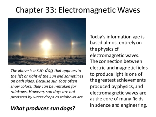
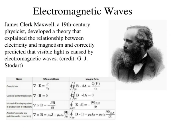
Physics 2113 Jonathan Dowling. Heinrich Hertz (1857–1894). Lecture 38: FRI 24 APR Ch .33 Electromagnetic Waves. Fields without sources?. Maxwell Equations in Empty Space:. Changing E gives B. Changing B gives E. Maxwell, Waves, and Light.

E N D
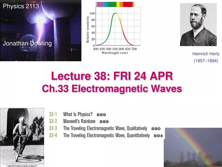
Physics 2113 Jonathan Dowling Heinrich Hertz (1857–1894) Lecture 38: FRI 24 APR Ch.33 Electromagnetic Waves
Fields without sources? Maxwell Equations in Empty Space: Changing E gives B. Changing B gives E.
Maxwell, Waves, and Light A solution to the Maxwell equations in empty space is a “traveling wave”… electric and magnetic fields can travel in EMPTY SPACE! The electric-magnetic waves travel at the speed of light? Light itself is a wave of electricity and magnetism!
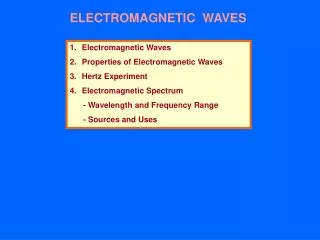
Electromagnetic waves First person to prove that electromagnetic waves existed: Heinrich Hertz (1875-1894) First person to use electromagnetic waves for communications: Guglielmo Marconi (1874-1937), 1909 Nobel Prize (first transatlantic commercial wireless service, Nova Scotia, 1909)
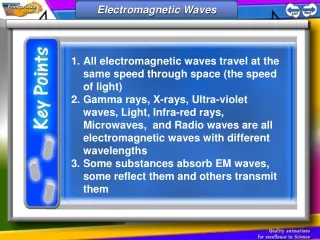
Electromagnetic Waves A solution to Maxwell’s equations in free space: Visible light, infrared, ultraviolet, radio waves, X rays, Gamma rays are all electromagnetic waves.
33.3: The Traveling Wave, Qualitatively: Figure 33-4 shows how the electric field and the magnetic field change with time as one wavelength of the wave sweeps past the distant point P in the last figure; in each part of Fig. 33-4, the wave is traveling directly out of the page. At a distant point, such as P, the curvature of the waves is small enough to neglect it. At such points, the wave is said to be a plane wave. Here are some key features regardless of how the waves are generated: 1. The electric and magnetic fields and are always perpendicular to the direction in which the wave is traveling. The wave is a transverse wave. 2. The electric field is always perpendicular to the magnetic field. 3. The cross product always gives the direction in which the wave travels. 4. The fields always vary sinusoidally. The fields vary with the same frequency and are in phase with each other.
Radio waves are reflected by the layer of the Earth’s atmosphere called the ionosphere. This allows for transmission between two points which are far from each other on the globe, despite the curvature of the earth. Marconi’s experiment discovered the ionosphere! Experts thought he was crazy and this would never work.
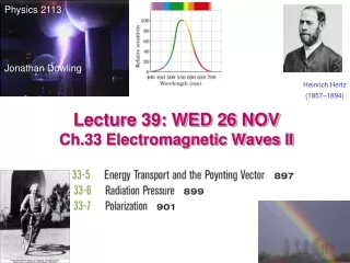
Electromagnetic Waves: One Velocity, Many Wavelengths! with frequencies measured in “Hertz” (cycles per second) and wavelength in meters. http://imagers.gsfc.nasa.gov/ems/ http://www.astro.uiuc.edu/~kaler/sow/spectra.html
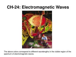
Maxwell’s Rainbow Fig. 33-2 Fig. 33-1 The wavelength/frequency range in which electromagnetic (EM) waves (light) are visible is only a tiny fraction of the entire electromagnetic spectrum. (33-2)
Next slide Oscillation Frequency: The Traveling Electromagnetic (EM) Wave, Qualitatively An LC oscillator causes currents to flow sinusoidally, which in turn produces oscillating electric and magnetic fields, which then propagate through space as EM waves. Fig. 33-3 (33-3)
33.3: The Traveling Wave, Quantitatively: The dashed rectangle of dimensions dx and h in Fig. 33-6 is fixed at point P on the x axisand in the xy plane. As the electromagnetic wave moves rightward past the rectangle, the magnetic flux B throughthe rectangle changes and—according to Faraday’s law of induction—induced electric fields appear throughout the region of the rectangle. We take E and E + dE to be the induced fields along the two long sides of the rectangle. These induced electric fields are, in fact, the electrical component of the electromagnetic wave.
33.4: The Traveling Wave, Quantitatively: Fig. 33-7 The sinusoidal variation of the electric field through this rectangle, located (but not shown) at point P in Fig. 33-5b, E induces magnetic fields along the rectangle.The instant shown is that of Fig. 33-6: is decreasing in magnitude, and the magnitude of the induced magnetic field is greater on the right side of the rectangle than on the left.
33.3: The Traveling Wave, Qualitatively: We can write the electric and magnetic fields as sinusoidal functions of position x (along the path of the wave) and time t : Here EmandBm are the amplitudes of the fields and,wand k are the angular frequency and angular wave number of the wave, respectively. The speed of the wave (in vacuum) is given by c. Its value is about 3.0 x10⁸ m/s.
Electric Field: Magnetic Field: Wavenumber: Wave Speed: Angular frequency: Vacuum Permittivity: Vacuum Permeability: Fig. 33-5 Amplitude Ratio: Magnitude Ratio: Mathematical Description of Traveling EM Waves All EM waves travel a c in vacuum EM Wave Simulation (33-5)