Download
1 / 41
410 likes | 435 Views
INDEXING SPATIAL DATABASES. Atinder Singh Department of Computer Science University of California Riverside , CA 92507. SPATIAL DATA

E N D
INDEXING SPATIAL DATABASES Atinder Singh Department of Computer Science University of California Riverside , CA 92507
SPATIAL DATA It can broadly be defined as data which covers multidimensional points,lines,rectangles, polygons, cubes and other geometric objects. Spatial data occupies a certain amount of space called it’s spatial extent, which is characterized by location and boundary. USES Geometric Information Systems. CAD/CAM Multimedia Applications Content based image retrieval Fingerprint matching MRI ( Digitized medical images)
TYPES OF SPATIAL DATABASESRegion Data: It has a spatial extent having a location and boundary. In two dimension the boundary can be defined as a line and in three dimension as surface. Region data basically is the geometric approximation to an actual data item. Example : Creating a rectangle encompassing any object such as a vehicle, house etc.Point Data: Point data consists of collection of points in a multidimensional space. It doesn’t cover any area. It can be based on direct measurements or be generated by transforming data obtained through measurements for ease of storage and querying. Example : Raster data is a directly measured data consisting of bitmaps and pixels maps of satellite imagery. Each pixel storing a measured value.
TYPES OF QUERIES1. Spatial range queries:They have an associated region and return a data that overlaps the region. Examples can be: find all cities within 50miles of LA or near 10 miles of the sea. Find all employees whose salary is between $40,000- $50,000 and age between 30-40.2. Nearest Neighbor queries: These queries are especially important for multimedia databases, where an object is represented by a point and similar objects are found by retrieving objects whose representative points are the closest to the one being queried. Example : Find cities nearest to LA.
3. Spatial Join queries :Typical example of such a query can be: “find all pair of cities within a range of 50miles of each other”, or, “find cities near lakes”. These queries can be most expensive to evaluate.
R Trees 1. Object Representation Objects in Spatial Databases are represented by a record entry of the form (I, tuple-identifier) in the R trees leaf nodes. I: is an n-dimensional rectangle bounding the spatial object indexed (‘n’ being the number of dimensions used). I is the closest bound over the object. tuple-identifier : is a unique identifier representing a tuple in the database b) The non-leaf nodes contain entries of the form (I, child-pointer) Child pointer is the address of a lower node in the tree like B trees and ‘I’covers all the rectangles encompassing its children's in the tree.
2. Main Features: Height Balanced trees similar to B-trees. The structure is completely dynamic as it supports object additions/deletions. Nodes correspond to pages on the disk. If M is the maximum number of entries in one node and m = M/2. Then ‘m’ specifies the minimum number of entries allowed in a node except for the root. Every non-leaf node has between ‘m’ and ‘M’ children unless it is the root. The root node has at least two children unless it is a leaf.
For each index record (I, tuple-id) in a leaf node, I is the smallest rectangle that spatially contains the n-dimensional data object. The tuple-id is a pointer to the actual data. For each (I, child-ptr) entry in a non-leaf node, I is the smallest rectangle that spatially contains the rectangles in the child nodes. The height of a R tree at the most is |logm N|-1.
3. SAMPLE DATABASE REPRESENTATION R1 R2 R3 R4 R5 R6 R7 R8 R9 R10 R11 R11 R12 R13 R14 R15 R16 R17 R18 R19 R4 R1 R 13 R11 R14 R3 R9 R8 R10 R2 R5 R12 R18 R7 R6 R16 R17 R19 R15
4. INSERTS • To insert a data entry E(I, p). • Find Position: • Set N to be root. If N is a leaf node, return N. • Select an entry ‘F’ in N whose FI needs least enlargement to accommodate EI. In case of ties, choose entry with smallest area. • Descend until a leaf node is reached by setting N to be the child node pointed to by F. • If the selected F in the leaf node has place for E, insert E; else, invoke Splitnode and split F to F and FF to include all old entries and E. • Propagate any changes upwards by invoking Adjust Tree. • Grow the tree length if Adjust Tree caused the root to split.
ADJUST TREE ALGORITHM • Ascends from the leaf node(L) adjusting upwards. • Set N=L. If L was split previously, set NN= LL where LL is the second split node. • If N is the root, stop. • Let P be parent node of N and EN be N’s entry in P. Adjust EN I so that it tightly encloses all entry rectangles in N. • If N has a partner NN resulting from an earlier split, create a new entry ENNI enclosing all rectangles in NN and include an entry ENN P pointing to NN in P. • If P in the above doesn't have any space, invoke Split node to produce P and PP. • Set N= P and NN=PP in case of a split and repeat the above mentioned steps until N = root.
5. SEARCH Given an R-tree with root T find all records whose rectangles overlap a search rectangle S. • If T is not a leaf, search all entries E in the node to determine whether EI overlaps S. • For all overlapping entries, invoke Search on the tree whose root node is pointed to by Ep. • If ‘T’ is a leaf, check all entries E to determine whether EI overlaps S. If so, E is a qualifying record. Unlike the B trees, a number of paths from the root will be followed while carrying out the search. It is thus not possible to guarantee a good worst case performance. The algorithm however eliminates following irrelevant regions of the indexed space.
6. DELETIONS Remove index record E from the R-tree. • Find node L containing the record E with T being root. • If T is not a leaf, check each entry F in T to determine if FI overlaps EI. For each such entry invoke the find process(Find leaf) on the tree whose root is pointed to by Fp until E is found or all nodes searched. • If T is a leaf, check each entry to see if it matches E. If found return T. • If no node is returned by step one stop. • Else remove E from L. • Invoke CondenseTree, passing L to it. • If the root has only one child after the tree has been adjusted, make the child the new root.
6a. CondenseTree • Given a leaf node L from where an entry has been deleted, set N=L. Set Q , a set of eliminated nodes to empty. • If N is the root, go to last step. • Else let P be the parent of N and let EN be N’s entry in P. • If N has fewer than m entries, delete EN from P and add the entries in N to set Q. • If N has not been deleted, adjust EN I to tightly contain all entries in N. • Set N=P and repeat from second step. • Re-insert all entries of nodes in set Q into the tree as described in Insert Algorithm. Entries from higher nodes are placed at their respective levels.
7. Node Splitting(Splitnode Algorithm) In order to add new entries to an already full node it is important to split it. The split should be done in a manner to make it unlikely as possible for both nodes to be searched for finding a particular entry. The aim is to minimize the covering area of the newly created nodes. There are three type of algorithms for splitting a node. Bad Split Good Split
7a. Exhaustive Algorithm • It is the most straight forward way to find the minimum area node split. It does that by generating all possible groupings and chooses the best. • The complexity of this algorithm is however very high even for moderate amount of nodes. It can go upto 2^M-1.
7b. Quadratic Cost Algorithm To divide a set of M+1 entries into two groups. • Apply algorithm PickSeedsto choose two entries to be the first elements of the group. • If all entries assigned Stop. • If one group has so few entries that all the rest must be assigned to it in order for it to have the minimum number ‘m’, assign the remaining to it. • Invoke Algorithm PickNext to choose the next entry to assign. • Add to the group whose covering rectangle will have to be enlarged least to accommodate it. • Resolve ties in the following manner • Group having smaller area • Fewer entries.
Pick Seeds Used to select the first two entries while splitting a node. • For each pair of entries E1 and E2, compose a rectangle J compromising of the both. • Calculate d = area(J) – area(E1 I) – area(E2 I) • Choose the pair with the largest d. This algorithm aims at choosing the pair of nodes which would have minimum overlap or are the farthest.
PickNext This algorithm picks the next node from the set Q. • For each entry E in Q and not yet inserted, Calculate d1 = The area increase required in the covering rectangle of the Group 1 to include E. d2 = The area increase required in the covering rectangle of the Group 2 to include E. • Choose an entry with the maximum difference between d1and d2. (Aim is to choose an entry with maximum preference for any one already created rectangle)
The quadratic algorithm aims to minimize the time required in finding the smallest area split at the cost of accuracy. The cost is quadratic in M.
7c.Linear-Cost Algorithm This algorithm is linear in M. The linear split is identical to Quadratic split but uses a different version of PickSeeds while PickNext chooses any of the remaining entries. The under mentioned algorithm is the LinearPickSeeds. • (Find extreme rectangles along all dimensions) Along each dimension find the rectangle having highest low side and the one having lowest high side. Record their separation. • Normalize by dividing the separation by the width of the entire set along the corresponding dimension. • Choose the pair with the greatest normalized separation along any dimension.
8. UPDATES AND OTHER OPERATIONS • In case a particular tuple is updated, it is deleted from the record, updated and re-inserted as a new record. Unlike B-trees, an updated record can find itself in a completely new location in the R-tree. • R-trees also support various other queries such as : finding all records in a particular range or all objects that contain a search area.
9. PARAMETERS AFFECTING PERFORMANCE • The area covered by a directory rectangle should be minimized. Here the aim is to reduce dead space ( Space covered by bounding rectangle but not covered by enclosed rectangle. • Overlap between directory rectangles should be minimized. This also decreases the number of paths required to be traversed for a query. • Margin of a directory rectangle should be minimized. Margin here is the sum of the sides of a rectangle. With fixed area, the smallest margin is that of a square. • Storage utilization should be minimized. Higher storage utilization can reduce query time as the height of the tree is reduced.
9. PROBLEM WITH R TREES • The main problem with R trees is that the parameters discussed affect each other in such a complex way, that optimizing one of them may result in the deterioration of the overall performance. • In implementing Quadratic split, if the algorithm starts with a small seed, if an object lies on the same axis as a seed it might be distributed early though being far away from the particular seed. A needle shape enlargement can take place having small bounding rectangle but large distance.
If one of the seeds happened to be enlarged, a new object might again be assigned to it as it would require comparatively lesser enlargement to enclose the new object. • If one of the groups has received very less entries all other entries are assigned to it. This may cause a very non-optimized expansion of that particular directory node.
R* TREE R* trees are a variant of R-trees which aim to improve performance keeping the parameters into mind. They are also a better indexing data structures for spatial joins ( map overlay structure) which are one of the most important operations in geographic and environmental databases. The R-trees versions take into consideration only the area parameter while making their decisions and optimizing the tree performance. Besides area R* trees also take into consideration the margin and overlap parameters. The major variation from original R trees lies in the manner it splits the overflow nodes.
The overlap of an entry can be defined as the sum of the overlap of the particular entry with all the objects of a node. If Ei….Ep are the entries in a node and Ek needs to be inserted, Overlap (Ek) = [i=1 to p && ik] area(Ek Ei )
10 INSERTION • Set N to the root. • If N is a leaf, return N. • Else :If the childpointers in N point to leaves determine the minimum overlap cost. • Choose the entry in N whose rectangle needs least overlap enlargement to include the new data rectangle. Resolve ties by choosing the entry requiring least area enlargement. • If the childpointers in N do not point to leaves determine the minimum area cost as in R-trees. • Set N to be the childnode pointed to by the child pointer of the chosen entry and repeat the above steps.
11. Split algorithm in the R*trees R*-trees uses more than the area criteria to choose a good split . It also looks into margins and overlaps and chooses an axis over which it carries out its split. The method used is: (Distribution method) • Along each axis the entries are first sorted by the lower value ,then by higher value. • For M+1 entries we can have M-2m+2 distributions of two nodes where ‘m’ is the minimum number of entries required in one node. The Kth distribution where K= 1…..M-2m+2 will have (m-1)+k entries and the second group will have the rest.
11. GOODNESS VALUE PARAMETERS • Goodness values based on area, margin and overlap are determined for each distribution. The algorithm chooses an axis based on the combination of these goodness values. The values are: • Area value: area[bb(first gp)] + area[bb(second gp)] • Margin value: margin[bb(first gp)] + margin[bb(second gp)] • Overlap value: area[bb(first gp)] area[bb(second gp)]
12. ALGORITHM SPLIT • Invoke Choose Split Axis to determine the axis perpendicular to which split is performed. • Invoke Choose Split Indexto determine the best distribution into two groups along that axis. • Distribute the entries into two groups.
ALGORITHM CHOOSE SPLIT INDEX • For each axis, Sort the entries by the lower and then by the upper value of their rectangles and determine all distributions as described above. • Compute ‘S’, the sum of all margin values of the different distributions. • Choose the axis with the minimum S as split axis.
ALGORITHM CHOOSE SPLIT-INDEX • Along the chosen axis , choose the distribution with the minimum overlap-value. • Resolve ties by choosing the distribution with minimum area value.
R7 An example R6 Y R5 R4 R3 R2 R1 X-axis
The split algorithm was tested with varying values of ‘m’. The values taken were 20%, 30%, 40%, 45%. This algorithm performs best with the value of 40%. • Cost: • For each axis the entries have to be sorted two times which requires O(M log(M)). • The cost of margin calculation will be carried out for 2(2*(M-2m+2)) rectangles. • The overlap cost will be that of calculating for 2*(M-2m+2)rectangles.
13. INSERTION ALGORITHM MODIFICATION The insertion algorithm of R* is the same as the R-tree except for it’s handling of overflow nodes. Here only the change carried out in case of a overflow is discussed. Overflow Treatment • If the level at which the overflow takes place is not at root level and it is it’s first call of Overflow in the given level invoke ReInsert else invoke Split.
ALGORITHM REINSERT • For all M+1 entries of the overflow node N, compute the distance between the centers of their rectangles and the center of the bounding rectangle of N. • Sort the rectangles in decreasing order of distances computed in the above step. • Remove first ‘p’ entries from N and adjust the rectangle of N. • In the chosen ‘p’ entries start with the maximum distance (=far insert ) or minimum distance(=close reinsert) and invoke insert algorithm to insert the entries. In the above algorithm the value of ‘p’ can be varied for leaf and non leaf nodes to achieve an optimum result. Experiments have shown that 30% is the ideal value of ‘p’.
ADVANTAGE OF RE-INSERT ALGORITHM The performance of the original R-tree would deteriorate with time as new entries are added. Rectangles at different levels of the tree created during early stages may not be suitable enough later on to ensure a good retrieval performance. To overcome this the Overflow algorithm aims to dynamically restructure tree structure to a point. The main advantages are: • Can change entries between neighboring nodes decreasing overlap • Can improve storage utilization. • More restructuring can cause less splits. • Since outer rectangles of a node are re-inserted, the shape of the directory rectangles can be more quadratic which is favorable.
TEST RESULTS The tests to measure performance of R* trees were carried out against different variants of R-trees( differing in Splits). The criteria chosen was to measure performance against the parameters mentioned above . The results showed that • R* tree is the most robust method. For every query file and data file less disc excess is required. • Gain in efficiency for small query rectangles was much higher than the large ones in whose case storage utilization becomes more important. • The maximum gain against other trees( linear, Greene’s and quadratic ) is between 400% to 180%. • R* proved to have the best storage utilization.
R+ TREES • This variation of R-trees aims at reducing the overlap of different entries at the rate of space utilization to decrease the search cost. It states that if a data entry is overlapping or extending into two upper non-leaf nodes, it should be divided into two half . G B A
PROPERTIES OF R+ TREES • For each entry (p, R) in an intermediate node, the sub tree rooted at the node pointed to by ‘p’ contains an entry S, if and only if S is covered by R. Exception being, if S is a rectangle at a leaf node. In this case S must just overlap with R. • For any two entries at the intermediate nodes, the overlap between their rectangles is zero. • Root has at least two children unless it is a leaf. • All leaves are at same level. • There is no constraint on the minimum number of entries at each node.