Download
1 / 12
120 likes | 305 Views
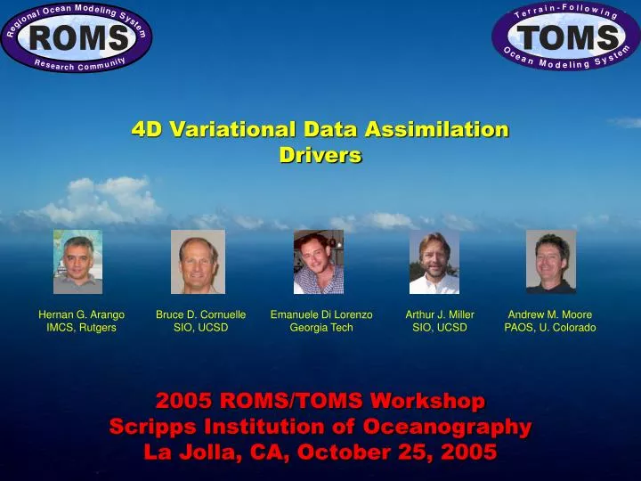
4D Variational Data Assimilation Drivers. Hernan G. Arango IMCS, Rutgers. Bruce D. Cornuelle SIO, UCSD. Emanuele Di Lorenzo Georgia Tech. Arthur J. Miller SIO, UCSD. Andrew M. Moore PAOS, U. Colorado. 2005 ROMS/TOMS Workshop Scripps Institution of Oceanography

E N D
4D Variational Data Assimilation Drivers Hernan G. Arango IMCS, Rutgers Bruce D. Cornuelle SIO, UCSD Emanuele Di Lorenzo Georgia Tech Arthur J. Miller SIO, UCSD Andrew M. Moore PAOS, U. Colorado 2005 ROMS/TOMS Workshop Scripps Institution of Oceanography La Jolla, CA, October 25, 2005
Objectives • To build 4D variational assimilation (4DVAR) platforms: • Strong Constraint S4DVAR • Conventional S4DVAR: outer loop, NLM, ADM • Incremental S4DVAR: inner and outer loops, NLM, TLM, ADM (Courtier et al., 1994) • Efficient Incremental S4DVAR (Weaver et al., 2003) • Weak Constraint W4DVAR (IOM) • Indirect Representer Method: inner and outer loops, NLM, TLM, RPM, ADM (Egbert et al., 1994; Bennett et al, 1997)
Tend Tstr How To Run • Run nonlinear model (NLM) and save background state trajectory at regular intervals over the desired data assimilation time window (FWDname) • Activate CPP options FORWARD_WRITE, FORWARD_RHS, andOUT_DOUBLE • Variational data assimilation CPP options: • S4DVAR Conventional strong constraint 4DVAR • IS4DVAR Incremental strong constraint 4DVAR • W4DVAR Weak constraint 4DVAR (BACKGROUND, FORWARD_READ, FORWARD_MIXING) • Set input parameter in s4dvar.in or w4dvar.in: • Descent algorithm parameters • Spatial convolution parameters (decorrelation scales) • Observation file names • First guess solution (background) file name
Metadata Dimensions: record Number of saved iteration survey Number of different time weight Number of interpolation weight datum Observations counter, unlimited dimension Variables: Nobs(survey) Number of observations per time survey survey_time(survey) Survey time (days) obs_type(datum) State variable ID associated with observation obs_time(datum) Time of observation (days) obs_lon(datum) Longitude of observation (degrees_east) obs_lat(datum) Latitude of observation (degrees_north) obs_depth(datum) Depth of observation (meters or level) obs_Xgrid(datum) X-grid observation location (nondimensional) obs_Ygrid(datum) Y-grid observation location (nondimensional) obs_Zgrid(datum) Z-grid observation location (nondimensional) obs_error(datum) Observation error, assigned weight obs_value(datum) Observation value NLmodel_value(record,datum) Nonlinear model interpolated value TLmodel_value(record,datum) Tangent linear model interpolated value Hmat(weight,datum) Interpolation weights
Observations NetCDF 8 7 5 6 4 3 1 2 (i2,j2,k2) (i1,j1,k1) dimensions: record= 2 ; survey= 1 ; weight= 8 ; state_variable= 7 ; datum = UNLIMITED ; // (79416 currently) variables: charspherical; spherical:long_name = "grid type logical switch" ; intNobs(survey) ; Nobs:long_name = "number of observations with the same survey time" ; doublesurvey_time(survey) ; survey_time:long_name = "survey time" ; survey_time:units = "days since 2000-01-01 00:00:00" ; survey_time:calendar = "365.25 days in every year" ; doubleobs_variance(state_variable) ; obs_variance:long_name = "global (time and space) observation variance" ; obs_variance:units = "squared state variable units" ; intobs_type(datum) ; obs_type:long_name = "model state variable associated with observation" ; obs_type:units = "nondimensional" ; doubleobs_time(datum) ; obs_time:long_name = "time of observation" ; obs_time:units = "days since 2000-01-01 00:00:00" ; obs_time:calendar = "365.25 days in every year" ; doubleobs_depth(datum) ; obs_depth:long_name = "depth of observation" ; obs_depth:units = "meter" ; doubleobs_Xgrid(datum) ; obs_Xgrid:long_name = "x-grid observation location" ; obs_Xgrid:units = "nondimensional" ; doubleobs_Ygrid(datum) ; obs_Ygrid:long_name = "y-grid observation location" ; obs_Ygrid:units = "nondimensional" ; doubleobs_Zgrid(datum) ; obs_Zgrid:long_name = "z-grid observation location" ; obs_Zgrid:units = "nondimensional" ; doubleobs_error(datum) ; obs_error:long_name = "observation error, assigned weight, inverse variance" ; obs_error:units = "inverse squared state variable units" ; doubleobs_value(datum) ; obs_value:long_name = "observation value" ; obs_value:units = "state variable units" ; doubleNLmodel_value(datum, record) ; NLmodel_value:long_name = "nonlinear model interpolated value" ; NLmodel_value:units = "state variable units" ; doubleTLmodel_value(datum, record) ; TLmodel_value:long_name = "tangent linear model interpolated value" ; TLmodel_value:units = "state variable units" ; doubleHmat(datum, weight) ; Hmat:long_name = "interpolation weights" ; Hmat:units = "nondimensional"
Processing • Use hindices, try_range and inside routines to transform (lon,lat) to (,) • Find how many survey times occur within the data set (survey dimension) • Count observations available per survey (Nobs) and assign their times (survey_time) • Sort the observation in ascending time order and observation time for efficiency • Save a copy of the observation file • Several matlab scripts to process observations
Ipass=1 Outer Loop CALL initial CALL main3d NLM: compute model-observations misfit and cost function CALL ad_initial CALL ad_main3d ADM: compute cost function gradients CALL descent CALL wrt_ini Compute NLM initial conditions using first guess conjugate gradient step size Ipass=2 CALL initial CALL main3d NLM: compute change in cost function Compute NLM initial conditions using refined conjugate gradient step size CALL descent CALL wrt_ini “Conventional” S4DVAR
Incremental S4DVAR CALL initial CALL main3d NLM: compute basic state trajectory and extract model at observations locations Outer Loop Ipass=1 Inner Loop TLM: compute misfit cost function between model (NLM+TLM) and observations CALL tl_initial CALL tl_main3d CALL ad_initial CALL ad_main3d ADM: compute cost function gradients Compute TLM initial conditions using first guess conjugate gradient step size CALL descent CALL tl_wrt_ini Ipass=2 CALL tl_initial CALL tl_main3d TLM: compute change in cost function Compute TLM initial conditions using refined conjugate gradient step size CALL descent CALL tl_wrt_ini Compute NLM new initial conditions (NLM+TLM) CALL ini_adjust CALL wrt_ini
Efficient Incremental S4DVAR CALL initial CALL main3d NLM: compute basic state trajectory and extract model at observations locations Outer Loop CALL ad_initial CALL ad_main3d ADM: compute initial estimate of the gradient CALL ini_descent Initialize conjugate direction as the negative of the gradient (adjoint) solution Inner Loop RPM: compute misfit cost function between model (NLM+TLM) and observations CALL tl_initial CALL tl_main3d CALL ad_initial CALL ad_main3d ADM: compute cost function gradients Compute TLM initial conditions using conjugate gradient step size CALL descent CALL tl_wrt_ini Compute NLM new initial conditions (NLM+TLM) CALL ini_adjust CALL wrt_ini
W4DVAR, IOM nl_roms: compute basic state trajectory nl_roms < nl_roms.in iom_roms: compute first guess and misfitbetween observation and model iom_roms < iom_roms.in Outer Loop Inner Loop ad_roms < ad_roms.in Inner loop, backward (ad_roms) and forward (tl_roms) integrations to compute tl_roms < tl_roms.in IOM components ad_roms: backward integration to compute ad_roms < ad_roms.in iom_roms < iom_roms.in iom_roms: compute
Final Remarks • It is running in parallel • Pre-conditioning, pre-conditioning … • Background term in cost function • Modeling of background error covariance • Efficient spatial convolution algorithms (3D implicit diffusion algorithms; parallelism) • Open boundary condition challenges • Quality control of observations • New observational data streams