Download

1 / 44
770 likes | 1.51k Views
Classical Planning and GraphPlan. Classes 17 and 18 All slides created by Dr. Adam P. Anthony. Overview. Planning as a separate problem Planning formalism Example p lanning problems Planning in State Space Planning Graphs GraphPlan Algorithm Other approaches.

E N D
Classical Planning and GraphPlan Classes 17 and 18 All slides created by Dr. Adam P. Anthony
Overview • Planning as a separate problem • Planning formalism • Example planning problems • Planning in State Space • Planning Graphs • GraphPlan Algorithm • Other approaches
Planning as a Separate Problem • Planning = Determining a sequence of actions to take that will achieve some goal(s) • Doesn’t that sound familiar? • That sounds similar to a search algorithm • Also, we could re-cast this idea using first-order logic • Key insight: planning domains are much more carefully structured and constrained than the general search/resolution problems • A customized algorithm will have better performance
Planning Domain Definition Language • PDDL is a factored representation • Entire world represented by variables • In essence PDDL defines a search problem: • Initial state • Actions (with preconditions) • Action results (post conditions) • Goal test/State • Similar to traditional language called STRIPS
Representing States • Use a language similar to FOL: • Poor ^ Unknown • At(Truck1, Melbourne) ^ At(Truck2, Sydney) • Difference #1 from FOL: Database semantics • Anything not mentioned presumed false (no negations needed/allowed) • Unique names certain to specify distinct objects • Difference #2: all facts are ground, and functionless • At(x,y) not permitted, nor is At(Father(Fred), Sydney) • Can be specified using logic notation (common) or with set semantics where fluents are categorized into groups that are manipulated using set operators Each fact is called a Fluent
Representing Actions • Actions are specified in terms of what changes • Anything not mentioned is presumed to stay the same • Uses an action schema • Limited FOL representation (all universally quantified) • Action name • Variable list • Precondition • Effect • Taking an action constitutes successfully grounding all the variables to literals that are true (or not) in the state At(here) ,Path(here,there) Go(there) At(there) , At(here)
Sample Action Action Schema: Action(Fly(p,from,to), PRECOND: At(p,from) Plane(p) Airport(from) Airport(to) Effect: At(p,from) At(p,to)) Actual (Grounded) Action: Action(Fly(P1,SFO,JFK), PRECOND: At(P1,SFO) Plane(P1) Airport(SFO) Airport(JFK) Effect: At(P1,SFO) At(P1,JFK)) Number of grounded Actions: O(Vk) where V is the number of variables in the action, k is the number of literals defined in the state
Applying Actions • An action is applicable if the preconditions are satisfied by some literals in the state S • Applying an action a in state S, has the result S’: • S’ = (S – Del(a)) Add(a) • Add(a): Add-list comprised of positive literals in a’s effects list • Del(a): Delete-list comprised of negative literals in a’seffects list • To remain consistent, we require that any variable in the effects list also appear in the preconditions list • Time is implicit in the language: Actions are taken at time T, and effects occur at time T+1
Planning Domains • A set of action schemas completely specifies a Planning Domain • A single Planning Problem includes all the schemas from the domain, plus an initial state and a goal • Initial state: any conjunction of ground atoms such that each atom either appears, or can be bound to a variable, in at least one precondition item for at least one action • Goal: Many ways of veiwing. Simplest: Action schema where goal test is the precondition and the effect is the ground literal: GoalAccomplished • Multiple Goals are covered by making one more goal in which accomplishing each goal is part of the precondition
Example Planning Domains • Cargo transport • Spare tire problem • Blocks World
Example: Cargo Transport • Reality: Fed-Ex and UPS • Simplification: • Actions = Load, Unload, Fly • Predicate: In(c,p): package c is in plane p • Predicate: At(x,a): Item (plane or package) is At airport a • Packages are no longer ‘at’ the airport, if they are ‘in’ the plane (to compensate for lack of universal quantifiers) • In Class: define the action schema
Example: Spare Tire Problem • Goal: restore a car to having 4 good tires • Fluents: Tire(Flat), Tire(Spare), Trunk, Axle, Ground • Predicate: At(x,y) • Actions: • Remove(obj, loc) • PutOn(obj,loc) • LeaveOvernight—all tires are stolen • In Class: define actions and discuss whether domain is realistic enough to be useful
B A C TABLE Example: Blocks world The blocks world is a micro-world that consists of a table, a set of blocks and a robot hand. Some domain constraints: • Only one block can be on another block • Any number of blocks can be on the table • The hand can only hold one block Typical representation: ontable(a) ontable(c) on(b,a) handempty clear(b) clear(c)
Blocks world operators • Here are the classic basic operations for the blocks world: • stack(X,Y): put block X on block Y • unstack(X,Y): remove block X from block Y • pickup(X): pickup block X • putdown(X): put block X on the table • Each will be represented by • a list of preconditions • optionally, a set of (simple) variable constraints • The effects, split into ADD and DEL: • a list of new facts to be added (add-effects) • a list of facts to be removed (delete-effects) • For example: preconditions(stack(X,Y), [holding(X), clear(Y)]) deletes(stack(X,Y), [holding(X), clear(Y)]). adds(stack(X,Y), [handempty, on(X,Y), clear(X)]) constraints(stack(X,Y), [XY, Ytable, Xtable])
Blocks world operators II operator(stack(X,Y), Precond [holding(X), clear(Y)], Constr [XY, Ytable, Xtable], Add [handempty, on(X,Y), clear(X)], Delete [holding(X), clear(Y)]). operator(pickup(X), [ontable(X), clear(X), handempty], [Xtable], [holding(X)], [ontable(X), clear(X), handempty]). operator(unstack(X,Y), [on(X,Y), clear(X), handempty], [XY, Ytable, Xtable], [holding(X), clear(Y)], [handempty, clear(X), on(X,Y)]). operator(putdown(X), [holding(X)], [Xtable], [ontable(X), handempty, clear(X)], [holding(X)]).
STRIPS planning • STRIPS: first major planning system out of SRI • STRIPS maintains two additional data structures: • State List - all currently true predicates. • Goal Stack - a push down stack of goals to be solved, with current goal on top of stack. • If current goal is not satisfied by present state, examine add lists of operators, and push operator and preconditions list on stack. (Subgoals) • When a current goal is satisfied, POP it from stack. • When an operator is on top stack, record the application of that operator on the plan sequence and use the operator’s add and delete lists to update the current state.
A C B A B C Typical BW planning problem Initial state: clear(a) clear(b) clear(c) ontable(a) ontable(b) ontable(c) handempty Goal: on(b,c) on(a,b) ontable(c) • A plan: • pickup(b) • stack(b,c) • pickup(a) • stack(a,b)
A C B A B C Another BW planning problem Initial state: clear(a) clear(b) clear(c) ontable(a) ontable(b) ontable(c) handempty Goal: on(a,b) on(b,c) ontable(c) • A plan: • pickup(a) • stack(a,b) • unstack(a,b) • putdown(a) • pickup(b) • stack(b,c) • pickup(a) • stack(a,b)
A B C C A B Goal state Goal interaction • Simple planning algorithms assume that the goals to be achieved are independent • Each can be solved separately and then the solutions concatenated • This planning problem, called the “Sussman Anomaly,” is the classic example of the goal interaction problem: • Solving on(A,B) first (by doing unstack(C,A), stack(A,B) will be undone when solving the second goal on(B,C) (by doing unstack(A,B), stack(B,C)). • Classic STRIPS could not handle this, although minor modifications can get it to do simple cases Initial state
A B C C A B Sussman Anomaly Achieve on(a,b) via stack(a,b) with preconds: [holding(a),clear(b)] |Achieve holding(a) via pickup(a) with preconds: [ontable(a),clear(a),handempty] ||Achieve clear(a) via unstack(_1584,a) with preconds: [on(_1584,a),clear(_1584),handempty] ||Applying unstack(c,a) ||Achieve handempty via putdown(_2691) with preconds: [holding(_2691)] ||Applying putdown(c) |Applying pickup(a) Applying stack(a,b) Achieve on(b,c) via stack(b,c) with preconds: [holding(b),clear(c)] |Achieve holding(b) via pickup(b) with preconds: [ontable(b),clear(b),handempty] ||Achieve clear(b) via unstack(_5625,b) with preconds: [on(_5625,b),clear(_5625),handempty] ||Applying unstack(a,b) ||Achieve handempty via putdown(_6648) with preconds: [holding(_6648)] ||Applying putdown(a) |Applying pickup(b) Applying stack(b,c) Achieve on(a,b) via stack(a,b) with preconds: [holding(a),clear(b)] |Achieve holding(a) via pickup(a) with preconds: [ontable(a),clear(a),handempty] |Applying pickup(a) Applying stack(a,b) From [clear(b),clear(c),ontable(a),ontable(b),on(c,a),handempty] To [on(a,b),on(b,c),ontable(c)] Do: unstack(c,a) putdown(c) pickup(a) stack(a,b) unstack(a,b) putdown(a) pickup(b) stack(b,c) pickup(a) stack(a,b) Goal state Initial state
Algorithms for Finding Plans in State Space • STRIPS is intuitive, but has problems because it is ‘working as it thinks’ • Let’s think of another method… • Planning algorithms have a start-state • Actions, if applicable, will change the state • Goal: easily tested by analyzing the current state for the given conditions • Sounds like a general search problem! • Why we wasted the time with PDDL: better heuristics
Forward Search • Start with initial state, apply any operators for which the preconditions are satisfied • Repeat on frontier nodes until you reach the goal • Problem: Lots of wasted time exploring irrelevant actions • Problem: Schema may be small, but adding more fluents exponentially increases the size of the state space • Not all hope is lost: heuristics will be very helpful!
Backward (Regression) Relevant-States Search • Similar in philosophy to STRIPS • Start with goal, search backward to start state • ONLY explore actions that are relevant to satisfying the preconditions of the current state • Difference: search algorithms and heuristics can prevent ‘sussman’s anomaly’ • Backward search requires reversible actions, but PDDL is good for that • Also needs to allow state SETS (since the goal may have non-ground fluents) • Unification of variables allows backward search to dramatically reduce branching factor vs. forward search • Set-based heuristics are harder to design.
Planning Heuristics • Key advantage of PDDL and planning as its own topic: effective problem-independent heuristics • Insight: PDDL problem descriptions all have a similar structure, independent of problem area • Makes forward search for many planning problems feasible • Common choices • Ignore preconditions • Ignore delete lists • Subgoal independence • Pattern Databases
A new view on heuristics • We’ve already discussed viewing search in a state space as a graph search problem: • One way of thinking about designing a heuristic is to add edges to the state space graph • Shorter paths mean shorter (admissible) estimates for cost to the goal
Ignoring Preconditions • Apply actions regardless of whether the state has satisfied the preconditions • Value of heuristic: minimum number of actions such that the union of their effects-sets equals the set of conditions in the goal • Sound Familiar? • Approximations are effective, but lose A* admissibility requirement • May also ignore only selected preconditions • But this is a domain-dependent heuristic
Ignoring Delete Lists • Assume goals and preconditions only have positive literals (easy to augment any problem—how?) • What happens then? • Remove delete lists • Executing one action never ‘undoes’ another • Applying any action monotonically increases toward the goal • FF Planner (Hoffman 2005) uses this heuristic with a modified hill climbing search that keeps track of solution path
Subgoal Independence • Assume that solving each of K items in the goal is independent of the others • Run K planning searches, one for each goal then sum the cost of each sub-plan to estimate cost of total plan • Optimistic Heuristic: when negative interactions occur between subplans (one undoes the other) • Admissible • Pessimistic Heuristic: when subplans contain redundant actions • Not admissible
Pattern Databases • Frequently Called Plan Libraries • Many planners are used repeatedly using new start states • Action schemas make this possible • Record exact solutions to plans and sub-plans as you solve them • Research questions: • Detecting frequently recurring and useful sub-plans • Using plan libraries to solve problems in a different domain • based on qualitative graph structures (Bulka, 2009)
Planning Graphs • Planning Graph: secondary data structure generated from a planning problem • Analyzing this data structure leads to a very effective heuristic • Approximates a fully expanded search tree using polynomial space • Estimates the steps to reach the goal • Always correct if goal not reachable • Always underestimates (so what?)
Planning Graph Basics • A planning Graph is divided into levels • Two types of alternating levels: • State levels Si fluents that MIGHT be true at level i • Always underestimates the time at which it will actually be true • Action levels AiActions that MIGHT be applicable at step i • Takes into consideration some but not all negative interactions between actions • Negative interaction = Performing one action violates the preconditions of the other • “The level j at which a literal first appears is a good estimate of how difficult it is to achieve the literal from the initial state [in the final plan].”
Example Problem and Planning Graph Initial State: Have(Cake) Goal State: Have(Cake) Eaten(Cake) Action(Bake(Cake) Pre: Have(Cake) Effect: Have(Cake)) Action(Eat(Cake) Pre: Have(Cake) Effect: Have(Cake)Eaten(Cake))
Constructing a Planning Graph • All action schemas must be propositionalized • Generate all possible grounded actions so no variables are left. • Start with S0 = all initially true fluents • Construct Ai = all actions whose preconditions are satisfied by Si • Construct Si = all fluents made true by the effects of the actions in Ai-1 • All levels in Aihave the NO-OPaction which passes all true fluents in Si to Si+1
Constructing a Planning Graph (Continued) • Add links: • Between levels • From fluents in Si to preconditions of actions in Ai • From effects of actions in Ai to fluents in Si+1 • Within Levels (mutual exclusion) • Action Mutex Link: Two actions compete for resources • State Mutex Link: Two fluents that cannot both be true at the same time
Rules for Constructing Mutex Links • Action Mutex: • Inconsistent Effects: One action negates the effect of the other (e.g., Eat(Cake) and Bake(Cake) ) • Interference: One of the effects of one action is the negation of a precondition of the other (e.g., Eat(Cake) and the persistence of Have(Cake)) • Competing Needs: One of the preconditions of one action is mutually exclusive with a precondition of the other • Depends on State Mutex links in previous level • State Mutex: • One is the negation of the other • All pairs of actions that could make both true have Acton mutex links between them
Example Problem and Planning Graph Initial State: Have(Cake) Goal State: Have(Cake) Eaten(Cake) Action(Bake(Cake) Pre: Have(Cake) Effect: Have(Cake)) Action(Eat(Cake) Pre: Have(Cake) Effect: Have(Cake)Eaten(Cake))
Growth of the Planning Graph • Levels are added until two consecutive levels are identical (graph has leveled off) • How Big is this Graph? • For a (propositionalized) planning problem with L literals and a actions, • Each Si level: Max L nodes, L2mutex links • Each Ai level: Max a + L nodes, (a + L)2mutex links • Inter-level linkage: L(a + L) links • Graph with n levels O(n(a+L)2)
Planning Graph Heuristics • If any goal literal fails appear, then the plan is not solvable • For a single goal: • Level at which it appears is a simple estimate for cost of achieving goal • Serial Planning Graphs insist that one action is performed at each level by adding mutex links between all non-NO-OP actions • Leads to more effective heuristic • For a conjunction of goals: next slide
Heuristics for Conjunction of Goals • Max-Level: Take the max of all goal literals • Admissible, but poorly conservative • Level-Sum: sum all goal costs together • not admissible but works OK much of the time • Set-Level: First level where all goal literals appear without Mutex links • Admissible, dominates Max-Level
Comments on Planning Graphs • Planning Graphs do have shortcomings: • Only guarantees failure in the obvious case • If goal does appear at some level, we can only say that there is ‘possibly’ a plan • In other words, there’s no obvious reason the plan should fail • Obvious reason = mutex relations • We could expand the process to consider higher-order mutexes • More accurate heuristics • Not usually worth the higher computational cost • Similar to arc-consistency in CSP’s
Extracting a (Possible) Solution • Implement as Backward-search • States = A level of the graph, and a set of goals • Start at level Sn, add all main goal fluents • Select a set of non-mutex actions that achieve the goals • Also, their preconditions cannot be mutex • New state is Level Sn-1 with its goals being the preconditions of the chosen action set • If we reach S0 with all goals satisfied, Success! • Heuristic: Solve the highest-level fluents first, using the lowest cost action (based on preconditions)
About No-Goods • no-goods is a hash table: • Store (level,goals) pairs • If Extract-solution fails it will: • Record its current goals and level in no-goods • If Extract-solution reaches the exact same state later, we can stop early and return FAILURE (or, backtrack to a different part of search) • No-Goods is important for termination • Can’t just say ‘planning graph leveled off so we’re done’ • Planning graphs grow vertically faster than horizontally • Some plans need more horizontal space to be solved • Extract Solutions is thorough • If a plan exists, it will find it • If it can’t find a new reason to fail at level Si then adding a level won’t help
Other Approaches • Boolean satisfiability • Propositionalize actions, goal • Add successor-state axioms • Add pre-condition axioms • Use SATPLAN algorithm to find a solution • Seems complex, but is very fast in practice • Situation Calculus • Similar to satisfiability above • Incoporates all of FOL, more expressive than PDDL • Partial Order Planners (Up Next!)