Download
1 / 16
160 likes | 296 Views
Moving knowledge to action. A Forward and Adjoint Neighborhood Scale Air Quality Model. Eduardo P. Olaguer Director, Air Quality Research Houston Advanced Research Center. Science and Policy Issues at Stake.

E N D
Moving knowledge to action. A Forward and Adjoint Neighborhood Scale Air Quality Model Eduardo P. Olaguer Director, Air Quality Research Houston Advanced Research Center
Science and Policy Issues at Stake • Nonlinear ozone chemistry near large sources may require very fine resolution to address. • Coarse models may bias regulatory decisions by misrepresenting the efficacy of controls. • Industrial point source emissions are uncertain by 1-2 orders of magnitude. • Near source human exposure to ozone and air toxics may be large during emission events.
HARC Air Quality Model • Neighborhood scale 3D Eulerian chemistry transport model customized for near source applications. • Parameterized clear sky photolysis rates. • Very high temporal (10-20 s) and spatial (100-400 m horizontal, 50 m vertical) resolution. • Forward and inverse (adjoint) model. • Coded in MATLAB to facilitate adjoint model. • Documented in 3 peer-reviewed publications (Atmos. Environ. and J. Air & Waste Manage. Assoc.). • Two manuscripts on chemical adjoint in review.
HARC Model Transport • Piecewise Parabolic Method for advection • Explicit scheme for horizontal diffusion • Uniform horizontal diffusion coefficient (can be adjusted by inverse model) • Semi-implicit (Crank Nicholson) scheme for vertical diffusion • Height-dependent vertical diffusion coefficient from similarity theory (3 stability classes)
HARC Chemical Mechanism • Total of 47 gas phase reactions (compared to 150 for CB05 and 260 for SAPRC07) • Detailed mechanisms for HCHO and highly reactive VOCs (ethene, propene, 1,3-butadiene, 1-butene, 2-butene, isobutene) • Truncated mechanisms for isoprene, toluene, xylenes • Less reactive (“background”) organics lumped together and assigned a total OH reactivity (rBVOC), where BVOC + OH HO2 + XO2. • Simplified chemical solver • Chemical equilibrium assumed for OH and HO2 (OK for NO > ~0.5 ppb) • EBI scheme (Hertel et al., 1993) for NO-NO2-O3 • Euler backward scheme for longer lived species (HONO, HCHO, CO, 6 olefins, ISOP, TOL, XYL, RNO3)
Mixing ratios of OH (left) and HO2 (right) at 10:00 – 15:00 CST, 9/14/2006 for rBVOC=0 (black), rBVOC=observed (blue), and TRAMP measurements (red), where rBVOC=total OH reactivity of unresolved organic species. Note: The HARC model performs similarly to standard mechanisms also compared against TRAMP data (Chen et al., 2012). As chemical interferences have been found in the Laser Induced Fluorescence (LIF) method used to measure HOx (Mao et al., 2012), the discrepancy between model predictions and true HOx concentrations are not as large as they appear.
Ozone NOx + ethene NOx + propene NOx + propene NOx + ethene NO2 NO NOx + ethene NOx + propene NOx + ethene Olefin NOx + propene Mixing ratios of O3, NO2, NO and olefin predicted by OZIPR model for the CB05 (black), SAPRC97 (red), and HARC (blue) mechanisms, with an initial 100 ppb olefin plume. Initial CO and NOx set at 200 ppb and 10 ppb.
Forward Modeling ofHouston Ship Channel Flare • 10-hr flare release of >14,000 lbs of ethene • Nearest downwind monitor 12 km away • Simulation resolution: 200 m x 200 m (horizontal) x 50 m (vertical) x 20 s (temporal) • Domain: 12 km x 12 km (horiz) x 1 km (vert) • Time period: 9:30 am – 12:30 am CST • Hourly varying uniform horizontal wind • Molar HCHO:CO = ~8% (TCEQ Flare Study)
200 m resolution Flare + Routine Flare only No primary HCHO 200 m resolution Observations 1 km resolution Flare + Routine 200 m resolution
Inverse Modeling of TexAQS IIFlare Emission Event • HCHO at Lynchburg Ferry (LF) peaked at 52 ppb on Sep 27, 2006 (Eom et al., 2008). • HCHO peak occurred during an olefin flare accompanying an 18-day sequential shutdown of a petrochemical facility ~8 km upwind of LF. • Performed 4Dvar inverse modeling of flare event emissions of CO, HCHO, olefins based on LF observations of NOx, O3, HCHO, olefins.
Horizontal Resolution: 400 m Horizontal Domain Size: 8 km × 8 km (BC and met obs)
Inverse Model Assumptions • Annual mean routine point source emissions • Link-based mobile emissions from MOVES courtesy of Houston Galveston Area Council • Inverse modeling for two cases of the HCHO upwind boundary condition: • Control: 4 ppb (typical in Houston urban air) • Sensitivity: 31.5 ppb (max at HRM-3 monitor) • Sensitivity run simulates transport of secondary HCHO from outside model domain
Inverse Modeling Results sensitivity run control Inferred HCHO event emissions: Control: 282 kg/hr Sensitivity run: 239 kg/hr Note: This is about 50 times larger than flare HCHO emissions from routine operations inferred during the 2009 SHARP campaign (Wood et al., 2012). LF observations Conclusion: Substantial event emissions of primary HCHO are required in addition to olefin emissions to explain LF observations.
Computer Aided Tomography (CAT) + DOAS 300 m Downtown Houston Moody Tower LP-DOAS LP-DOAS light paths 130 m 70 m 20 m 5.15 km 5.08 km 4.1 km
U=2 m/s Single point source E = 10 g/s Kh =13.2 m2/s Neutral stability CAT reconstruction using Algebraic Reconstruction Technique and 2T90° DOAS configuration with 20 light rays. 3-hr forward model results with “true” parameter values 30 min assimilation window First Guess: E = 1 g/s Kh =132 m2/s Optimized: E = 9.3 g/s Kh =16.2 m2/s CAT-4Dvar reconstruction based on 2T90° Error of improved reconstruction
Future Work • Link to micro-scale CFD or WRF LES model to simulate air flow with realistic buildings. • Combine with chemical fingerprinting tools (e.g., Positive Matrix Factorization). • Perform short-range (~2 km) CAT-DOAS for reactive HAPs (e.g., toluene and xylenes) during BEE-TEX field study in Houston in 2014. • Apply CAT-DOAS to longer-range (~10 km) measurements of HCHO, HONO, NO2, SO2, O3.