Download
1 / 34
340 likes | 347 Views
Overview of Atmospheric Reanalysis. Prehistory. Pencil, paper, knowledge such as geostrophic winds, fonts, cyclones (1957 Carter County Tornado, 5/21/57). First Use of Computers. Need 3-Dimensional analysis for initial conditions for numerical weather models

E N D
Prehistory Pencil, paper, knowledge such as geostrophic winds, fonts, cyclones (1957 Carter County Tornado, 5/21/57)
First Use of Computers Need 3-Dimensional analysis for initial conditions for numerical weather models Value at grid point was a weighted mean of the nearby observations Better methods based on the same theme: Cressman analysis, Optimal Interpolation However, a good hand drawn map was better! It’s the knowledge factor. - geostrophic winds - thermal winds - fronts - Norwegian cyclone model - …
Big Step Forward: 3D-Var Typically an analysis has more degrees of freedom than number of observations. There is no unique solution. The next approach was to look at it as an inverse problem. Realize that there many solutions but you need to get an answer by adding a constraint. Best constraint? Finding the analysis which minimized the cost function.
3D-Var: Constraints Constraint #1 Observations – want analysis to be close to observations (H(x) – yO)T(E+R)-1(H(x) –yO) Constraint #2 First guess – a forecast made from the previous analysis (typically 6 hours before) – want analysis to be close to the first guess. (x-xb)TB-1(x- xb) Constraint #3 Statistics: anomaly (obs-first guess) => nearby points, B is not diagonal Constraint #4 Physics:
Height Observation: height field X +ve height Obs – First Guess isobars from Statistics
Height Observation: wind field X +ve height Obs – First Guess Wind Field based on Statistics Northern Hemisphere
3D-Var: Constraints Constraint #1 Observations – want analysis to be close to observations (H(x) – yO)T(E+R)-1(H(x) –yO) Constraint #2 First guess – a forecast made from the previous analysis (typically 6 hours before) – want analysis to be close to the first guess (x-xb)TB-1(x- xb) Constraint #3 Statistics: anomaly (obs-first guess) => nearby points, B is not diagonal Constraint #4 Physics:
Inverse Problem: 3D-Var Constraint #4 Physics: geostrophic winds: deviation from non-linear balance (SSI) RH between 0 and 100 (GSI, weak) dry mass conservation (GSI)
The Time Had Come for Reanalysis Suggestions: Bengtsson and Shukla (1988), Trenberth and Olson (1988) 3D-Var: SSI (NCEP) late 80’s, early 90’s 3D-Var was a good theoretical basis for making analyses still using basic theory, still using cost function some details have changed from late 1980s to now ex. old “B” is function of latitude, new: function of flow 3D-Var: first guess = 6 hour forecast (3 dimensional) Assumed that obs took place at the at the analysis time Improvements such as FGAT 4D-Var: first guess → trajectory in phase space (3D + time) Observation time is used appropriately
First Reanalyses: ECMWF: ERA-15 period covered:1979-1993 based on ~1995 operational system, OI stopped because of change in computer, 3D-Var/FGAT available NASA/DAO: NASA/DOA Reanalysis period covered: 1980-1995, 3D-multivariate OI NCEP: NCEP/NCAR Reanalysis period covered 1948-present based on ~1993 operational system, 3D-Var (SSI) Cray X-MP, Power chips, Linux, new system every 3-5 years still being used at CPC, and outside 4270 results from Google Scholar for 2016 2006: JMA,CRIEPI: JRA-25, JCDAS (real-time), 3D-Var period: 1979-2014 replaced by JRA-55
First Reanalyses: Results Atmospheric state, radiative fluxes, atmospheric water cycle, soil moisture. Gold mine of data: 10,000s of scientific papers shipping, power, insurance, agriculture, health Google scholar: N/N R=45K results Google: N/N R=225K results NCEP Infrastructure: ieee files → grib1 files (BAMS CD with GrADS, wgrib) NO NCEP web sites: no web distribution of model output → pre-nomads (internet) public distribution data: little → cd → dvd + internet (nomads) Most important? Some money was spent on recovering old observations. Afterwards people realized the importance and continued recovery. Integration of datasets: Antarctic scientists wondered why the NCEP/NCAR Reanalysis had biases in the older analyses. Importance of GTS (Global Telecommunication System): don’t put your obs onto GTS, they don’t get used by the operational meteorological centers and Reanalyses.
First Reanalyses: Problems NCEP/NCAR Reanalysis perspective Low resolution (order 250 km) meant that some problems could not be addressed. Radiation code was expensive, so only run every 3 hour (6 hours in some other reanalyses). So you could have rain and sun. (Radiation code was run before the rain started.) Soil moisture Polar regions Stratosphere (use of sigma vertical coordinates) Spurious trends most common is going from no obs to obs in 1948 (start) only continental USA and parts of Europe no obs: analysis climatology resembles model climatology satellite data
Modern Reanalyses: ECMWF: ERA-Interim 4D-Var, 1979-present program: hierarchy of reanalyses JMA: JRA-55 4D-Var, 1958-present JRA-55C (conventional) 1972-2012 GMAO/NASA: MERRA-1, MERRA-2 3D-Var MERRA-1 1979-2016, MERRA-2 1979-present NCEP: CFSR 3D-Var, ocean+atmosphere, 1979-present ESRL/NOAA: 20th Century Reanalysis v2 1871-2012 only assimilates surface pressure (with SST forcing)
Modern Reanalyses: The modern reanalyses (aside from 20th Century) have improved resolution, better models, and better data assimilation systems. Haven’t solved the issue of spurious climate changes when new satellite systems are introduced. In one modern reanalysis, the problems with satellite-induced “climate” changes were worse than their first reanalysis. 20th Century Reanalysis: only assimilate surface pressure! Very long record (1871-2012) No problems with spurious climate shifts caused by satellite data Fewer problems with changes in the network Biases in the instruments .. not bad But “No Free Lunch” – not as accurate
Current Reanalyses: Trends are still a problem Reanalyses are very useful; however, spurious trends is still a big problem. Big spurious trends in the real-time analyses from changes in real-time systems (model and data assimilation) were eliminated. Reanalyses got rid of the big problem but little problems remained. This is a problem because climate trends are also little. #1 Biases in the observations Satellites, sondes, SST #2 Changes in Observation Density No observations – analysis climatology resembles model climatology Many observations – analysis resembles observations 1950's except for a few places, no obs .. resembles model climo 2017 many obs, obs less biased, resembles reality Fix: better models, more efficient assimilation techniques
Ex. Using an Older System Observation Rich Region Z200 box-average Time series
Trends of Box-Average Z200 for Observation Rich Region Time series of box average of Z200 in CONUS Should be easy to estimate trend: box average, observation rich Reanalyses with satellite obs → ??? trends Reanalyses without satellite obs → more consistent Using satellite observations to produce trends is not a solved problem. Conventional observations has problems too! Changes in instrumentation can introduce biases. Care has to be used when using trends from reanalyses.
Future Themes: Near Term Heirarchy of reanalysis: Multiple reanalyses: Surface obs: surface pressure Surface pressure + winds Advantages: long record, time consistency Disadvantages: not as accurate Conventional obs: Advantages: 1950s-present No problems from satellite data Disadvantages: not as accurate as satellite based analyses All observations including satellites: Advantages: most accurate analysis as measured by forecast skill score Disadvantages: satellites can cause spurious climate shifts ECMWF: major project JMA: JRA-55, JRA55C NOAA: 20th Century v3, R1 replacement, GEFS reanalysis, CFSv3
Future Themes: Long Term Hierarchy of reanalysis: Combined oceanic and atmospheric reanalysis Problem: deep ocean takes hundreds of years to equilibrate * Earth system reanalysis Problem: deep ocean takes hundreds of years to equilibrate mountain glaciers take hundreds of years to equilibrate * ice sheets take thousands of years to equilibrate * * K. McGuffie A. Henderson-Sellers, 2005
CORe Questions Do we need satellite data for climate monitoring? Avoiding satellite data will improve trends What cost in accuracy? Where do you need satellite data? SH? Stratosphere? Enough accuracy for Climate Monitoring? Forecast initial conditions: need best accuracy Climate monitoring: trade some accuracy for better trends Simple test: as good as R1 in reproducing a modern (satellite) reanalysis (ERA-interim).
Summary for 1979-2010 CORe CORe = experimental data assimilation conventional observations + non-radiance satellite obs using Ensemble Kalman Filter data assimilation Often better than NCEP/NCAR reanalysis (compared to ERA-interim) Even in the data poor SH and lower stratosphere. NCEP/NCAR Reanalysis and other reanalyses show effects of introducing new satellite observations. CORe doesn't assimilate radiance observations which are the cause of many trend problems. So if CORe is of sufficient accuracy for the particular application, it may be better as it hasn't the problems with the introduction of new satellites. Still have other sources of errors in the trends: observation network isn't fixed, biases in the observations. However, a conventional data assimilation is good for much of the climate monitoring that CPC does.
Selecting a Reanalysis Many reanalyses are available: how to choose? Period of record? Spatial resolution? Legal restrictions? What data are assimilated? * surface obs? Long record length, noisy, * conventional data? Medium record length, noisy? * satellite observations? Familiarity? Yours, others Use more than one reanalysis if possible.
Using a Reanalysis Reanalyses come in several formats. National Meteorological Centers usually use grib, a WMO format. NASA uses HDF. Universities tend to use NetCDF. While at CPC, you are welcome to use CPC's archive of reanalyses. /cpc/cfsr/reanalyses/ Contact Leigh Zhang. Era-Interim, ERA5, ERA40 – must not be redistributed. JRA-55, JRA55c, JRA-25 – must not be redistributed. (need permission from ECMWF or JMA) You are welcome to make copies of the others.