Download

1 / 34
340 likes | 482 Views
Review of Expected Values. Review of Expected Values. Random Variable (RV) : Outcome of an experiment Value unknown until experiment is completed Expected Value of Random Variable X, E(X): Also known as the Mean Value

E N D
Review of Expected Values • Random Variable (RV): Outcome of an experiment • Value unknown until experiment is completed • Expected Value of Random Variable X, E(X): • Also known as the Mean Value • Weighted average of the values of the RV where weights are the associated probabilities Probability Density Function (PDF)
Review of Expected Values • Expected Value of a Function of RV’s, g(X) • Lets define g(X) ≡ [X-E(X)]2 • s2≡ E[g(X)] = E[[X-E(X)]2] • Known as RV Variance [Var(X)] PDF E(X)
Review of Expected Values • Var(x) is a measure of dispersion or spread of a distribution • → E(x2)=s2 +µ2 • σ≡ standard deviation of x
Review of Expected Values • y = α + βx RV constants • E(y) = α + βE(x) • Var(y)=E(y2)-[E(y)]2 = E(α2 + 2αβx + β2x2)-[E(α + βx)]2 = α2 + 2αβE(x) + β2E(x2) - α2 - 2αβE(x) - β2[E(x)]2 = β2E(x2)-β2[E(x)]2 = β2[E(x2)-[E(x)]2] = β2[E(x2)-µ2] = β2 Var(x)=Var(y) • Variance of a constant times a RV is the square of the constant times var(RV) y y2
Expectations with a Joint Distribution • Two RV’s, X and Y • Joint distribution (PDF), f(x,y) • Means and Variances defined via the use of marginal distributions, fx(x) and fy(y) • Discrete: fx(x)=yf(x,y), fy(y)=xf(x,y) • Continuous: fx(x)=∫yf(x,y)dy, fy(y)=∫xf(x,y)dx • For discrete case: E(x)=Σxxfx(x)=Σxx(Σyf(x,y)) = ΣxΣy x f(x,y) • For continuous case: • E(x)=∫xxfx(x)dx=∫x∫yxf(x,y)dydx fx(x)
Expectations with a Joint Distribution • Lets define function g(X,Y) • Covariance measures how RV’s move together • A function of 2 RV’s • Cov(x,y) = σxy ≡ E[(x-µx)(y-µy)] E(X) E(Y)
Expectations with a Joint Distribution • σxy ≡ E[(x - µx)(y - µy)] • when y=x, σxy = σxx =E[(x- µx)2] • σxy=E[xy-xE(y)-yE(x)+E(x)E(y)] = E(xy) -E[xE(y)] -E[yE(x)]+E(x)E(y) = E(xy) -E(x)E(y) • -E(y)E(x)+E(x)E(y) • =E(xy) - E(x)E(y) • =E(xy) - μxμy
Expectations with a Joint Distribution • Given its definition, if σxy> 0 → x and y tend to be above (below) their means at the same time • σxy< 0 → x and y tend to be above (below) their means at different times • I would like to show that if f(x,y) =fx(x) fy(y) → σxy=0 • I will assume the joint PDF equals the product of the marginal PDF’s
Expectations with a Joint Distribution • If f(x,y)=fx(x) fy(y)→σxy=0 ? • σxy= E[(x - µx)(y - µy)]→ = E(x - μx)E(y - μy)=0*0 • → σxy = 0 if f(x,y)=fx(x)fy(y) f(x,y) expected value of deviations from mean
Expectations with a Joint Distribution • Correlation coefficient, r, where –1<r<1 • Standardized covariance term • where σx, σy>0 • ρ has same sign as σxy • More linearly related, larger || value • ||=1→x,y are perfectly correlated • Unit-free measure
Expectations with N RV’s • Let X represent an (N x 1) vector of RV’s • How can we represent the covariances of these N RV’s (Σ)? N x N (N x N) σii ≡V(Xi) = variance of Xi σij≡cov(Xi,Xj) = covariance of Xi and Xj
Expectations with N RV’s • Characteristics of Σ • Σ is a symmetric matrix (σij = σji) i≠j • Σ is positive semi-definite • DEF: Symmetric matrix A (N x N) is positive definite if and only if w′Aw>0 for all w≠0N (w is (N x 1) vector) • DEF: Symmetric matrix A is positive semi-definite if and only if w′Aw≥0 for all w≠0N • If at least one RV’s has a non-zero covaricance and there are no exact linear relationships between RV’s → Σ is positive definite
Expectations with N RV’s • Expected Values and Variances of • Linear Functions of N RV’s • X: (Nx1) vector of RV’s X1,…,XN A: (1 x N) vector of constants • →E[AX] = E[a1X1 + a2X2 + ... + anXn] = a1 E[X1] + a2 E[X2] + ... + aN E[XN] = a1μ1 + a2 μ2 + ... + an μN =Aμ(μ is a [N x 1] vector of means) elements of A elements of X (1 x 1) (1 x 1)
Expectations with N RV’s • This implies the variance of a linear function of RV’s can be obtained via the following: • V(AX) = E[(AX - E[AX])2 ] = E[{A(X-E[X])}2 ] = E[A(X-E[X])(X-E[X])'A'] • = A E[(X-E[X])(X-E[X])']A' • = AΣ A' =a scaler with A being (1 x N) and Σthe (N x N)covariance matrix = E[(X-E(X))(X-E(X))']
Expectations with N RV’s • What if we have the following function? • e.g., g(X1,X2) = X1±X2 • V(X1 ± X2)= Var(X1)+ Var(X2) ± 2Cov(X1,X2) • V(X1 ± X2)= Var(X1) + Var(X2) if Cov(X1,X2)=0 • Variance of a sum (difference) is the sum of the variances plus (minus) 2 times the covariances
Expectations with N RV’s • Lets extend this to a more complex example • X is a column vector of NRV’s • A and b are constant matrices • That is, we transform N random variables into m new random variables (Y)
Expectations with N RV’s • V(Y) is symmetric, positive- semi-definite matrix
Conditional Expectations • Conditional Density: • f(y|x) = f(x|y) = • x and y independent if f(y|x)=fy(y), f(x|y)=fx(x) • f(x,y) = f(x|y)fy(y) = f(y|x)fx(x) • Conditional Expectation:
Unconditional Expectation • Unconditional Expectation: • Expected value of g(x,y), e.g., Exy[g(x,y)] • = Ey [Ex|y g(x,y)]=Exy[g(x,y)]
Characteristics of RV’s With a Normal Distribution • Single RV: x~N(m,s2) • Characteristics: • Mean (µ) = median = mode • Variance is s2 • Normal distribution is symmetric about its mean and bell shaped • PDF has inflection points at x=m s
Characteristics of RV’s With a Normal Distribution • Noted below, a RV that is normally distributed is completed described by 2 statistics: mean (μ) and standard deviation (σ) • The PDF of a normally distributed RV, x [e.g., x~N(μ,σ2)] can be represented via the following:
Characteristics of RV’s With a Normal Distribution • If we standardize x, we obtain the standard normal PDF where x~N(μ, σ2)] : x* is std. normal RV
Characteristics of RV’s With a Normal Distribution • Linear functions of normally distributed RV’s are also normally distributed • x~N(µ, σ2), y = α + βx • →y~N(?,?) →y~N(α + βμ,β2σ2) • Let α = -µ/σ, β=1/σ • →z≡y~N(0,1), std. normal RV • With d>c, Pr(c<X<d)=Φ(z2)-Φ(z1) • z1=(c-µ)/σ, z2=(d-µ)/σ • Φ≡standard normal cumulative distribution function (CDF) constants
Characteristics of RV’s With a Normal Distribution • Extension to Multivariate Distribution • General overview • Marginal and conditional multivariate normal dist.
Characteristics of RV’s With a Normal Distribution • If we have 2 RV’s, x and y, that are distributed joint normal, the PDF looks like the following: • Note: The marginal distributsions of 2 RV’s are themselves normal • fx(x)=N(μx,σ2x), fy(y)=N(μy,σ2y)
Characteristics of RV’s With a Normal Distribution • Assume we have N RV’s and we represent these N RV’s via X • The N-dimension joint density f(X), where X has a mean vector, μ, and covariance matrix, Σ, can be represented via the following: (N x 1) (1 x N) (N x N)
Characteristics of RV’s With a Normal Distribution • If we let R represent the (N x N) correlation matrix, where • This implies • where X* is the standardized X value inverse of R
Characteristics of RV’s With a Normal Distribution • If all variables are uncorrelated, ρij=0, which implies R = IN, then the joint PDF can be represented as: • If in addition to being uncorrelated, σi =1 and μ=0 e.g., X~N(0,1)
Characteristics of RV’s With a Normal Distribution • N Random Variables • Partition into 2 subsets • X' =[x1 x2]~N(μ, ) • x1 is (N1 x 1), x2 is (N2 x 1) • μi is (Nix 1), is (N x N) • Σij is (Ni x Nj) N1+N2=N
Characteristics of RV’s With a Normal Distribution • Lets represent the conditional distribution of a subset of the N normally distributed RV’s via the following • E(x1|x2)=μ12 where • μ12=μ1+Σ12Σ22-1(X2-μ2) • V(x1|x2)=Σ11,2 where • Σ11,2=Σ11- Σ12 Σ22-1 Σ21 • x1|x1~N(μ12, Σ11,2) x2|x1~N(μ21, Σ22,1) (N1 x N2) (N2 x 1) (N1 x 1) (N2 x N2)
Characteristics of RV’s With a Normal Distribution • 2 Random Variables • X' =[x1 x2]~N(μ, ) • x2|x1~N(E[x2|x1], σ22(1-2)) E[x2|x1] a linear function of x1 • =0→x1 and x2 statistically independent →f(x2|x1,=0)=f(x2) →x2|x1~N(μ2, σ22) Var(xi) reduced variance
Characteristics of RV’s With a Normal Distribution • Assume we have M RV’s that are distributed multivariate normal: • Let D be a (T x M) matrix of constants where T ≤ M T x 1 T x 1 T x T
Other Distributions Of Interest • Chi-Square (c2) • If z~N[0,1]→x = z2~χ2(1df) • If z1, z2, …,zn are independent standard normal RV’s (e.g., zi~N[0,1])→ y=z12+z22+…+zn2 ~ χ2(n df) • t-distribution • Assume z~N[0,1], y~ χ2(r df) and are independent of one another • T=z/[(y/r)1/2] ~ t(r df) • Symmetric but more “flat” than standard normal • F-distribution • Assume z1~χ2(r1 df) and z2~χ2(r2 df) • y=(z1/r1)/(z2/r2) ~ F(r1,r2)