Download
1 / 53
530 likes | 604 Views
Lecture 6.1. Paolo PRINETTO Politecnico di Torino (Italy) University of Illinois at Chicago, IL (USA) Paolo.Prinetto@polito.it Prinetto@uic.edu www.testgroup.polito.it. Combinational design: the basic approach. Goal.

E N D
Lecture 6.1 Paolo PRINETTO Politecnico di Torino (Italy)University of Illinois at Chicago, IL (USA) Paolo.Prinetto@polito.it Prinetto@uic.edu www.testgroup.polito.it Combinational design:the basic approach
Goal • This lecture presents the basic approach to manual synthesis of Combinational networks.
Prerequisites • Modules 4 and 5, and Lecture 2.1
Homework • No particular homework is foreseen
Further readings • No particular suggestion
Outline • Manual synthesis approaches • Manual synthesis steps
User'sRequirements Logic level design system RT logic Impl behavior structure physical
=? =? =? =? Specification Specification Design Design rules rules =? =? =? =? User'sRequirements Implementation Implementation Step #1: Specification preparation system RT logic Specs behavior structure physical
=? =? =? =? Specification Specification Design Design rules rules =? =? =? =? User'sRequirements Implementation Implementation Step #1: Specification preparation system RT logic Specs System level, behavioral description behavior structure physical
=? =? =? =? Specification Specification Design Design rules rules =? =? =? =? User'sRequirements Implementation Implementation Step #2: Specification validation =? system RT logic Specs behavior structure physical
=? =? =? =? Specification Specification Design Design rules rules =? =? =? =? Implementation Implementation Step #3: Synthesis system RT logic Specs Impl behavior structure physical
=? =? =? =? Specification Specification Design Design rules rules =? =? =? =? Implementation Implementation Step #3: Synthesis system RT logic Specs Logic level, physical domain netlist description Impl behavior structure physical
Manual synthesis approaches • Several approaches are possible, not necessarily strictly each other orthogonal. • They could be classified as follows: • Purely manual • Partially automated • Partitioning based.
Purely manual approach • Karnaugh map based • When performing a manual synthesis it is: • rather easy to minimize the maximum delay (by designing 2-logic-level circuits, only) • extremely hard to minimize the area, trading off with the maximum delay.
Purely manual approach (cont’d) • Applicable when dealing with very few PIs, only (PIs 6) • It will be presented in the sequel of this lecture.
Partially automated approach • Some of the sub-steps can be accomplished resorting to tools freely downloadable from the web • Applicable when the behavior of each PO has been described by a Boolean Function expressed as a set of cubes
Partially automated approach • Some of the sub-steps can be accomplished resorting to tools freely downloadable from the web • Applicable when the behavior of each PO has been described by a Boolean Function expressed as a set of cubes • No significant limitation w.r.t. the # of PIs. • It will be presented in lecture 6.4.
Partitioning-bases approach • The system is first partitioned in functional blocks • Each functional block is then implemented resorting to one of the above mentioned approaches • The system is eventually designed simply assembling the functional blocks
Partitioning-bases approach • The system is first partitioned in functional blocks • Each functional block is then implemented resorting to one of the above mentioned approaches • The system is eventually designed simply assembling the functional blocks • No significant limitation w.r.t. the # of PIs • It will be presented in lecture 6.5
Partitioning-bases approach (cont’d) • Historically this method was thoroughly applied in the 70’s and 80’s when digital systems were mainly implemented by PCBs and the chips available were mostly the RT level basic blocks presented in lecture 5.2 and 5.3.
Outline • Manual synthesis approaches • Manual synthesis steps
Manual synthesis steps • Manual synthesis is usually performed in several sub-steps.
Step #3.1: Logic level refinements system RT logic Specs behavior structure physical
Step #3.1: Logic level refinements system RT logic Specs behavior structure physical
Step #3.1: Logic level refinements U = A’B’ + A D Boolean function of each PO system RT logic Specs behavior structure physical
Step #3.1: Logic level refinements • It’s usually performed in 2 sub-sub-phases:
Step #3.1.1: 1st refinements system RT logic Specs behavior structure physical
Step #3.1.1: 1st refinements Non-minimal Boolean function of each PO system RT logic Specs behavior structure physical
Usually accomplished by drawing the Karnaugh mapof each PO 00 01 11 10 00 1 0 - 0 01 1 0 - 1 11 1 0 - - 10 1 0 - - AB CD Step #3.1.1: 1st refinements Non-minimal Boolean function of each PO system RT logic Specs behavior structure physical
Step #3.1.2: Logic minimization system RT logic behavior structure physical
Step #3.1.2: Logic minimization Minimized Boolean function of each PO system RT logic behavior structure physical
Step #3.1.2: Logic minimization U = A’B’ + A D Minimized Boolean function of each PO system RT logic behavior structure physical
Note • A detailed analysis of manual logic refinements will be presented in lecture 6.2 whereas some algorithmic approaches will be introduced in lecture 6.3
Step #3.2: Library binding system RT logic behavior structure physical
Step #3.2: Library binding system RT logic behavior structure physical
A’ B’ U A D Step #3.2: Library binding system RT logic Netlist of ideal gates behavior structure physical
Step #3.2: Library binding • The library binding of sp expressions is trivial: • logicoperation logic gate • sum or • product and • complement not
Example • U = A’B’ + AD
Example • U = A’B’ + AD U
Example • U = A’B’ + AD U A D
Example • U = A’B’ + AD A’ U B’ A D
Example • U = A’B’ + AD A B U A D
Multiple outputs • When dealing with multiple outputs, shared implicants are naturally mapped in shared gates.
Example • X = b’d + bcd • Y = bd’ + bcd
Example Shared implicant • X = b’d + bcd • Y = bd’ + bcd
Example Shared implicant • X = b’d + bcd • Y = bd’ + bcd Shared gate b’ d X b c d Y b d’
Step #3.3: Technology mapping system RT logic behavior structure physical
Step #3.3: Technology mapping system RT logic behavior structure physical
Step #3.3: Technology mapping system RT logic Netlist of actual gates behavior structure physical