Download
1 / 31
310 likes | 418 Views
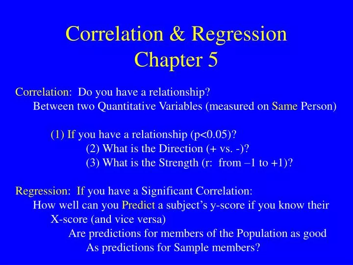
Correlation & Regression Chapter 5. Correlation : Do you have a relationship? Between two Quantitative Variables (measured on Same Person) (1) If you have a relationship (p<0.05)? (2) What is the Direction (+ vs. -)? (3) What is the Strength (r: from –1 to +1)?

E N D
Correlation & RegressionChapter 5 • Correlation: Do you have a relationship? • Between two Quantitative Variables (measured on Same Person) • (1) If you have a relationship (p<0.05)? • (2) What is the Direction (+ vs. -)? • (3) What is the Strength (r: from –1 to +1)? • Regression: If you have a Significant Correlation: • How well can you Predict a subject’s y-score if you know their • X-score (and vice versa) • Are predictions for members of the Population as good • As predictions for Sample members?
Correlations measure LINEAR Relationships No Relationship: r=0.0 Y-scores do not have a Tendency to go up or down as X-scores go up You cannot Predict a person’s Y-value if you know his X- Value any better than if you Didn’t know his X-score Positive Linear Relationship: Y-scores tend to go up as X-scores go up
Correlations measure LINEAR Relationships, cont. • There IS a relationship, but its not Linear • R=0.0, but that DOESN’T mean that the two variables are • Unrelated
Interpreting r-values • Coefficient of Determination – r2: • Square of r-value • r2 * 100 = Percent of Shared Variance; the Rest of the variance • Is Independent of the other variable r=0.50 r=0.6928
Interpreting r-values • If the Coefficient of Determination between height and weight • Is r2=0.3 (r=0.9): • 30% of variability in peoples weight can be Related • to their height • 70% of the difference between people in their of weight • Is Independent of their height • Remember: This does not mean that weight is partially • Caused by height • Arm and leg length have a high coefficient of • Determination but a growing leg does not cause • Your arm to grow
IV & DV both Quantitative • Correlation: • Each data point represents Two • Measures from Same person. • Is There a Relationship? • What Direction is the Relationship? • How Strong is the Relationship? • -1 0 1 • The stronger the relationship, • the better you can predict • one score if you know the • other. Rr=0.0 r=0.0 r=0.4 R=0.6 0.8 r=0.8 r=0.6 r=0.9 r=0.9 r=0.95
Negative Correlation • Quasi-Independent Variable: • # of cigarettes/day • Dependent Variable: • Physical Endurance • The fatter the field, the weaker • the correlation r=-0.50 r=-0.30 r=-090 r=-0.70 r=-0.95 r=-0.95 r=-0.99
Correlations # of Malformed Cells in Lung Biopsy # of Cigarettes Smoked per Day x 10
Correlation Lung Capacity # of cigarettes smoked per day x 10
Methodology: Restriction of Range • Restriction of Range cases an artificially low (underestimated) • value of r. • E.G. using just high GRE scores represented by the open circles. • Common when using the scores to determine Who is used in the • correlational analysis. • E.G.: Only applicants with high GRE scores get into • Grad School.
Computing r Raw Scores Deviation Scores
Computing r, cont. Z-scores
Methodology: Reliability • An instrument used to measure a Trait (vs. State) must be Reliable. • Measurements taken twice on the same subjects should agree. • Disagreement: • Not a Trait • Poor Instrument • Criterion for Reliability: r=0.80 • Coefficient of Stability: • Correlation of measures taken more than 6mo. apart
Regression • Creates a line of “Best Fit” running through the data • Uses Method of Least Squares • The smallest Squared Distances between the Points and • The Line • Y-hat = a +b*X and y= a +b*X-hat • a=intercept b=slope • The Regression Line (line of best fit) give you a & b • Plug in X to predict Y, or Y to predict X
Regression, cont. • Method of Lest Squares: • Minimizes deviations from regression line • Therefore, minimizes Errors of Prediction
Regression, cont. • Correlation between X & Y = Correlation between Y & Y-hat • Error of Estimation: Difference between Y and Y-hat • Standard Error of Estimation: sqrt (Σ(Y-Y-hat)2/n) • Remember what “Standard” means • The higher the correlation: • The lower the Standard Error of Estimation • Shrinkage: Reduction in size of correlation between sample • correlation and the population correlation which it measures
Multiple Correlation & Regression • Using several measures to predict a measure or future measure • Y-hat = a + b1X1 + b2X2 + b3X3 + b4X4 • Y-hat is the Dependent Variable • X1, X2, X3, & X4 are the Predictor (Independent) Variables • College GPA-hat = a + b1H.S.GPA + b2SAT + b3ACT + b4HoursWork • R = Multiple Correlation (Range: -1 - 0 - +1) • R2 = Coefficient of Determination (R*R * 100; 0 - 100%) • Uses Partial Correlations for all but the first Predictor Variable
Partial Correlations The relationship (shared variance) between two variables when the variance which they BOTH share with a third variable is removed Used in multiple regression to subtract Redundant variance when Assessing the Combined relationship between the Predictor Variables And the Dependent Variable. E.G., H.S. GPA and SAT scores.
Step-wise Regression • Build your regression equation one dependent variable at a time. • Start with the P.V. with the highest simple correlation with the DV • Compute the partial correlations between the remaining PVs and • The DV • Take the PV with the highest partial correlation • Compute the partial correlations between the remaining PVs and • The DV with the redundancy with the First Two Pvs removed. • Take the PV with the highest partial correlation. • Keep going until you run out of PVs
Step-wise Regression, cont. • Simple Correlations with college GPA: • HS GPA =.6 • SAT =.5 • ACT =.48 (but highly Redundant with SAT, measures same thing • Work =-.3 • College GPA-hat = a + b1H.S.GPA + b2SAT + b3HoursWork + b4ACT
Shrinkage • Step 1: Construct Regression Equation using sample which has • already graduated from college. • Step 2: Use the a, b1, b2, b3, b3 from this equation to Predict • College GPA (Y-hat) of high school graduates/applicants • The regression equation will do a better job of predicting College • GPA (Y-hat) of the original sample because it factors in all the • Idiosyncratic relationships (correlations) of the original sample. • Shrinkage: Original R2 will be Larger than future R2s
Forced Order of Entry • Specify order in which PVs are added to the regression equation • Used to test (1) Hypotheses and to control for (2) Confounding Variables • E.G.: Is there gender bias in the salaries of lawyers? • Point-Biserial Correlation (rpb) of Gender and Salary: rpb =0.4 • Correlation between Dichotomous and Continuous Variable • But females are younger, less experienced, & have fewer years • on current job • Create Multiple Regression formula with all the other variables • Then Add the test variable (Gender) • Look at R2: Does it Increase a lot or little at all? • If R2 goes up appreciably, then Gender has a Unique Influence
Other Types Of Correlation • Pearson Product-Moment Correlation: • Standard correlation • r = Ratio of shared variance to total variance • Requires two continuous variables of interval/ratio level • Point Biserial correlation (rpbs or rpb): • One Truly Dichotomous (only two values) • One continuous (interval/ratio) variable • Measures proportion of variance in the continuous variable • Which can be related to group membership • E.g., Biserial correlation between height and gender
Discriminant Function AnalysisLogistic Regression • Look at relationship between Group Membership (DV) and PVs • Using a regression equation. • Depression = a + b1hours of sleep + b2blood pressure • + b3calories consumed • Code Depression: 0 for No; 1 for Yes • If Y-hat >0.5, predict that subject has depression • Look at: • Sensitivity: Percent of Depressed individuals found • Selectivity: Percent of Positives which are Correct
Discriminant Function AnalysisLogistic Regression Four possible outcomes for each prediction (Y-hat): Y = 0 Y = 1 Sensitivity % Hits Y-hat < 0.5 Y-hat > 0.5 • Selectivity % Correct Hits
Discriminant Function AnalysisLogistic Regression • Expect Shrinkage: • Double Cross Validation: • Split sample in half • Construct Regression Equations for each • Use Regression Equations to predict Other Sample DV • Look at Sensitivity and Selectivity • If DV is continuous look at correlation between Y and Y-hat • If IVs are valid predictors, both equations should be good • Construct New regression equation using combined samples
Discriminant Function AnalysisLogistic Regression • Can have more than two groups, if they are related quantitatively. • E.G.: Mania = 1 • Normal = 0 • Depression = -1
Which Procedure To Use? • Logistic Regression produces a more efficient regression equation • Than does Discriminant Function Analysis: • Greater Sensitivity and Selectivity