Download
1 / 26
260 likes | 384 Views
A Loosely Coupled Ocean-Atmosphere Ensemble Assimilation System. Tim Hoar, Nancy Collins, Kevin Raeder, Jeffrey Anderson, NCAR Institute for Math Applied to Geophysics Data Assimilation Research Section.

E N D
A Loosely Coupled Ocean-Atmosphere Ensemble Assimilation System. Tim Hoar, Nancy Collins, Kevin Raeder, Jeffrey Anderson, NCAR Institute for Math Applied to Geophysics Data Assimilation Research Section Steve Yeager, Mariana Vertenstein, GokhanDanabasoglu, Alicia Karspeck, and Joe Tribbia NCAR/NESL/CGD/Oceanography AMS – 26 Jan 2011
Ocean Data Assimilation Motivation The resulting high-fidelity ocean states are needed. The ensembles provide uncertainty quantification. • Climate change over time scales of 1 to several decades has been identified as very important for mitigation and infrastructure planning. • High fidelity ocean states will be needed by the IPCC decadal prediction program. • The ocean plays a crucial role by providing a source or sink (and system memory) for the atmosphere of many quantities, such as heat, moisture, CO2, etc. • Increasing numbers of observations from larger regions of the oceans are making state-of-the-art data assimilation a promising possibility. AMS – 26 Jan 2011
Ensemble Filter For Large Geophysical Models 1. Use model to advance ensemble (3 members here) to time at which next observation becomes available. Ensemble state estimate, x(tk), after using previous observation (analysis) Ensemble state at time of next observation (prior) AMS – 26 Jan 2011
Ensemble Filter For Large Geophysical Models 2. Get prior ensemble sample of observation, y = h(x), by applying forward operator h to each ensemble member. Theory: observations from instruments with uncorrelated errors can be done sequentially. AMS – 26 Jan 2011
Ensemble Filter For Large Geophysical Models 3. Get observed value and observational error distribution from observing system. AMS – 26 Jan 2011
Ensemble Filter For Large Geophysical Models • 4. Compute the increments for the prior observation ensemble • (this is a scalar problem for uncorrelated observation errors). Note: Difference between various ensemble filters is primarily in observation increment calculation. AMS – 26 Jan 2011
Ensemble Filter For Large Geophysical Models 5. Use ensemble samples of y and each state variable to linearly regress observation increments onto state variable increments. Theory: impact of observation increments on each state variable can be handled independently! AMS – 26 Jan 2011
Ensemble Filter For Large Geophysical Models 6. When all ensemble members for each state variable are updated, there is a new analysis. Integrate to time of next observation … AMS – 26 Jan 2011
Experiment Overview Compare the effect of using a single atmospheric boundary vs. an ensemble of atmospheric boundaries on ocean data assimilation with POP. • “23 POP 1 DATM” denotes the experiment using 23 POP members and a single “data” atmosphere (CESM framework). • “48 POP 48 CAM” denotes the loosely coupled experiment using 48 POP members and 48 consistent but unique CAM atmospheres. • Both experiments were conducted for 1998 & 1999. • The 48 POP 48 CAM experiment was subsequently chosen to produce initial conditions for the IPCC decadal prediction program. AMS – 26 Jan 2011
Coupled Ocean-Atmosphere Schematic Obs used by NCAR-NCEP reanalyses CESM1 coupler history files: atmospheric forcing DART/CAM assimilation system DART/POP assimilation system Hadley + NCEP-OI2 SSTs World Ocean Database Observations CAM analyses: CAM initial files; posterior ensemble mean of state variables prior ensemble mean of all other variables CLM restart files; prior ensemble mean of all variables CICE restart files; prior ensemble mean of all variables POP analyses: temperature, salinity, velocities, surface height CAM state variables = PS, T, U, V, Q, CLDLIQ, CLDICE Prior = values before assimilation (but after a short forecast) Posterior = values after the assimilation of observations at that time AMS – 26 Jan 2011
Atmospheric Reanalysis Assimilation uses 80 members of 2o FV CAM forced by a single ocean (Hadley+ NCEP-OI2) and produces a very competitive reanalysis. O(1 million) atmospheric obs are assimilated every day. 500 hPa GPH Feb 17 2003 Generates additional ocean spread. Each POP ensemble member is forced with a different atmospheric reanalysis member. AMS – 26 Jan 2011
World Ocean Database T,S observation counts These counts are for 1998 & 1999 and are representative. FLOAT_SALINITY 68200 FLOAT_TEMPERATURE 395032 DRIFTER_TEMPERATURE 33963 MOORING_SALINITY 27476 MOORING_TEMPERATURE 623967 BOTTLE_SALINITY 79855 BOTTLE_TEMPERATURE 81488 CTD_SALINITY 328812 CTD_TEMPERATURE 368715 STD_SALINITY 674 STD_TEMPERATURE 677 XCTD_SALINITY 3328 XCTD_TEMPERATURE 5790 MBT_TEMPERATURE 58206 XBT_TEMPERATURE 1093330 APB_TEMPERATURE 580111 • temperature observation error standard deviation == 0.5 K. • salinity observation error standard deviation == 0.5 msu. AMS – 26 Jan 2011
Experimental Configurations • 23 POP 1 DATM • POP 1-degree displaced pole; • 23 ensemble members starting from a ‘climatological’ state; • Single ‘data’ atmosphere from CORE; • DART assimilates observations once per day in a +/- 12 hour window centered at midnight; • The CESM framework is responsible for all model advances. • The 48 POP 48 CAM experiment differed in that: • 48 ensemble members starting from a ‘climatological’ state; • Atmospheric forcing from the DART/CAM ensemble reanalysis; • Guide to the following figures: • Ensemble mean 1-day lead forecast difference from observations. • is # observations available; +,+ is # assimilated. • Obs are rejected if too far from ensemble mean (3 std dev here). AMS – 26 Jan 2011
Ensemble Spread for 100m XBT (Expendable Bathythermograph) • Spread contracts too much for 23 POP 1 DATM; • Using single atmospheric forcing is also part of the problem; • Model bias adds to the problem; • DART Statistical Sampling Error Correction also helps. Pacific Atlantic AMS – 26 Jan 2011
Ensemble Spread for Pacific 100m XBT Spread of the “climatological” ensemble In general, larger spread rejects fewer obs Twice as much! Small spread! AMS – 26 Jan 2011
Ensemble Spread for Atlantic 100m XBT In general, larger spread rejects fewer obs Twice as much! Small spread! AMS – 26 Jan 2011
10m Mooring Temperature RMSE • Ensemble mean 1-day lead forecast difference from observations. • is # observations available. +,+is # assimilated. • Observations are rejected if they are too far from ensemble mean • (3 standard deviations here). Pacific Atlantic AMS – 26 Jan 2011
10m Mooring Temperature RMSE – Pacific Ensemble mean 1-day lead forecast difference from observations. Similar observation rejection characteristics POP/CAM as good or better RMSE AMS – 26 Jan 2011
100m Mooring Temperature RMSE • 1/3 of the obs are still rejected by 48 POP 48 CAM in the Pacific. • Model bias in the thermocline? Pacific Atlantic AMS – 26 Jan 2011
100m Mooring Temperature RMSE – Pacific Many observations still not assimilated POP/CAM as good or better RMSE AMS – 26 Jan 2011
Physical Space: 1998/1999 SST Anomaly from HadOI-SST • POP forced by observed atmosphere (hindcast) Coupled Free Run 48 POP 48 CAM 23 POP 1 DATM AMS – 26 Jan 2011
Learn about ensemble assimilation and DART tools at: http://www.image.ucar.edu/DAReS/DART/ Anderson, J., Hoar, T., Raeder, K., Liu, H., Collins, N., Torn, R., Arellano, A., 2009: The Data Assimilation Research Testbed: A community facility. BAMS, 90, 1283—1296, doi: 10.1175/2009BAMS2618.1 AMS – 26 Jan 2011
End of Presentation, following slides held in reserve. AMS – 26 Jan 2011
Observation Visualization Tools AMS – 26 Jan 2011
Observation Visualization Tools AMS – 26 Jan 2011
The CAM-DART-POP Implementation Uses the CESM1 software framework; ocean, atmosphere, and other components communicate through the coupler. A few minor script changes and use of the interactive ensemble capability permit each member of an ensemble of POPs to be forced by a different CAM atmosphere. Once the additional files are staged, the basic implementation is a trivial addition to the run script that invokes the DART system. # ------------------------------------------------------------------ # See if CSM finishes correctly (pirated from ccsm_postrun.csh) # ------------------------------------------------------------------ # DART assimilation operating on restarts # ------------------------------------------------------------------ grep 'SUCCESSFUL TERMINATION' $CplLogFile if ( $status == 0 ) then ${CASEROOT}/assimilate.csh endif AMS – 26 Jan 2011