The Agencies Method for Modeling Coalitions and Cooperation in Games

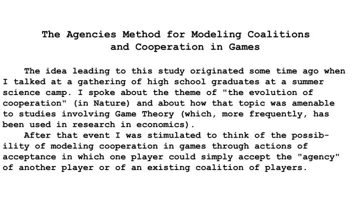
1. The Agencies Method for Modeling Coalitions and Cooperation in Games The idea leading to this study originated some time ago when I talked at a gathering of high school graduates at a summer science camp. I spoke about the theme of "the evolution of cooperation" (in Nature) and about how that topic was amenable to studies involving Game Theory (which, more frequently, has been used in research in economics). After that event I was stimulated to think of the possib-ility of modeling cooperation in games through actions of acceptance in which one player could simply accept the "agency" of another player or of an existing coalition of players.

2. The action of acceptance would have the form of being entirely cooperative, as if “altruistic”, and not at all competitive, but there was also the idea that the game would be studied under circumstances of repetition and that every player would have the possibility of reacting in a non-cooper-ative fashion to any undesirable pattern of behavior of any another player. Thus the game studied would be analogous to the repeated games of "Prisoner's Dilemma" variety that have been studied in theoretical biology. These studies of "PD" (or "Prisoner's Dilemma") games have revealed the paradoxical possibility of the natural evolution of cooperative behavior when the interacting organisms or species are presumed only to be endowed with self-interested motivations, thus motivations of a non-cooperative type.

3. Games in Theory and Games Played by Humans I feel, personally, that the study of experimental games is the proper route of travel for finding "the ultimate truth" in relation to games as played by human players. But in practical game theory the players can be corporations or states; so the problem of usefully analyzing a game does not, in a practical sense, reduce to a problem only of the analysis of human behavior. It is apparent that actual human behavior is guided by complex human instincts promoting cooperation among individuals and that moreover there are also the various cultural influ-ences acting to modify individual human behavior and at least often to influence the behavior of humans toward enhanced cooperativeness.

4. Our study has the character of an experiment, but rather than working directly with human subjects we computationally discover the evolutionarily stable behavior of a triad of bargaining or negotiative players. And these players are, as far as the experimental science is concerned, equivalent to a set of three robots. So whether or not the experiment can be carried out successfully becomes simply a matter of the mathematics. These computations are found to be “heavy” so that our research could not have been done in the earlier days of game theory, like in the 50’s, because of the inadequacy of the computing resources then. (And for the future we envision the feasibility of the study of much more complicated models for 4, 5, or more players, with many more distinct strategy parameters being involved.)

5. Demands and Acceptance Probabilities in the Case of Two Players We first worked out the function of players’ “demands” controlling their “probabilities of acceptance” (in a repeated game context) for the case of games of a simple bargaining type of two players. We present an explanation of this to prepare for and facilitate explaining the modeling structure for three (or more) players. Originally, in our first trials of the new ideas, we studied a model bargaining problem where the set of accessible possibilities was enclosed by a parametrically described algebraic curve (forming the Pareto boundary). This was arranged so as to have a natural bargaining solution point at (u1=1/2, u2=1/2) (referring to the players’ utility functions).

6. The total bargaining problem was asymmetric, but modulo the theory of localized determination of the solution point, it was such that (u1,u2) = (1/2,1/2) should be the compromise bargain. (We were surprised, however, when we found that if we used (as described below) different “epsilon numbers” (see below) for the players that that difference would unbalance the model’s selection of a bargaining solution (!). Later, thinking about it, we realized that the use of appropriately matching epsilon numbers for the players could be naturally justified. In a game problem with transferable utility (like with our studies for 3 players) this amounts to using THE SAME epsilon number for all players.) For Player 1 we let d1 stand for his demand (number) and e1 for his epsilon-number. The “epsilons” make the “reactive” behavior of a player depend smoothly on the numbers that the players choose as parameters of strategy so that we can obtain the system of equations to be solved for the equilibria by

7. differentiating a player’s expected payoff function with respect to each of the strategy parameters that that player controls. Then his “acceptance rate” a1 is defined in terms ofthese numbers plus also the data number u1b2 which is “the amount of utility that Player 1 is given by the Player 2 when Player 2 has become the agent for both of the players (and has selected a point on the Pareto boundary)” (and this data is observable by Player 1 simply through the known history of Player 2’s behavior in the repeated game).

8. We need a specific rule of relationship between d1 and a1 and this is (was) specified by the relations: A1 = Exp[ (u1b2 – d1)/e1 ], and a1 = A1/(1+A1) . (Which formulae have the effect that A1 is positive and that a1 is like a positive probability, between 0 and 1.) In a completely dual fashion, for Player 2, we specify: A2 = Exp[ (u2b1 – d2)/e2 ], and a2 = A2/(1+A2) .

9. As we remarked already, we discovered from the calculations that we needed to use e1 = e2 if we wanted desirable results! (But it seems that this can be justified as “impartial” if we consider another means for introducing probabilistic uncertain-ty affecting the consequences of demands; in particular, if the uncertainty resulted from “fuzziness” about the knowledge of the precise location of the Pareto boundary then that version of ignorance would affect the players in an impartial fashion.) In the case of two players the players would simultaneously vote, with each player voting either to accept the other as the general agent or voting, in effect, for himself/herself instead. Then our first idea was to apply an “election rule” declaring that an election was void if both of the players voted for accepting (the other player) and only effective if only one player made a voting choice of acceptance.

10. So then we specified that the election should be repeated with a certain probability (say probability (1-e4)) whenever both players had voted acceptance votes (and if that retrying process ultimately failed then the players finally were given the null reward {0,0} (in utilities) for failure to cooperate!). This complicated the “payoff formula” somewhat but the VECTOR of payoffs, {PP1,PP2}, was ultimately calculable as functionally dependent on a1, a2, u1b2, and u2b1. (In this listing the utility amounts were regarded as resulting from STRATEGY CHOICES by the players where P1 would actually choose {u1b1,u2b1} as a point chosen BY P1 (!) on the Pareto boundary curve. So, from the curve, u1b1 could be interpreted as a function of u2b1, with P1 interpreted as simply choosing u2b1 strategically.)

11. The vector {PP1,PP2} becomes a function of a1, a2, u1b2, u2b1, u1b1, and u2b2. And this reduces to the 4 quantities first listed because of u1b1 and u2b2 being determined by the Pareto curve. And a1 is a function of d1 and u1b2 with a2 similarly controlled by d2 and u2b1. So, ultimately, we arrive at 4 equations in four variables for the conditions of equilibrium. These derive from the partial derivatives of the payoff function for a player taken with respect to the parameters describing his strategic options. Thus there are the partial derivatives of PP1 with respect to d1 and with respect to u2b1 and these are both to vanish. Then there are two dual equations derived from PP2. (Later we learned that differentiating PP1 with respect to a1 directly, rather than viewing a1 as a function of d1, would give a simplified (but equivalent) version of the d1-associated equation.)

12. Graphics and Illustrative Data We interrupt the explanation, in the main text, of the mathematics of the model design to give descriptions relating to the six “Figures” which are placed later just before the references. These “Figures” illustrate the results achieved by the “experimental mathematics” work, that is, by our calculations developed in the project work. Fig. 1 shows how the “Pareto efficiency” of equilibrium solutions varies as the parameter e3 (which modulates the smoothness of the variation of an “acceptance probability”, like a1f23, as a function of the associated “demand parameter”, like d1f23). The calculations to find the points for the graph were carried through by A.K. (Alexander Kontorovich) for the case where e3 varies. e4 and e5 are fixed at 1/4, and the game

13. Fig. 2 is similar or parallel to Fig 1 but was worked out later, by S.L. (Sebastian Ludmer). This graph is derived from a game with only a symmetry between P1 and P2, and these are the “favored” players since, regarding the coalitions, v(1,2) = 2/3, while the other two-player coalitions have no value. And e3 varies while e4 and e5 are both set arbitrarily at 1/100. The same pattern (of improving efficiency) appears on this graph and it is easy to see that the ASYMPTOTIC level of the payoff-obtaining efficiency of the players at equilibrium is 100 per cent. Fig. 3 shows three graphs relating to three versions of “payoff prediction” according to three different sources. First there is the classical “Shapley value”, which becomes simply a line in this Figure, graphed in blue, second is the “prediction” derivable from the nucleolus, graphed in green, and third is the result of equilibria based on our model, graphed in pink.

14. For each individual graph, of the three, the quantity plotted in relation to the vertical axis is an “imbalance” measure that evaluates the extent to which the two more favored players, P1 and P2, get more payoff than P3. This is calculated as Imbalance = p1 + p2 – 2*p3 with the notation being that pk is the payoff received by player Pk, for k = 1,2,3. Players P1 and P2 are favored and symmetrically situated in this game where v(1,2) = b3 and the other two coalitions of two players are without any payoff value. The “imbalance” is charted as the function with values according to the vertical scale while the value of b3 = v(1,2) relates to the horizontal axis and scale. Fig. 3 was derived from calculations and graphics work of S.L. You will notice on Fig. 3 that the data presentation ends for b3 > 0.7 (roughly). What happened, actually, was that as we continued the finding of a family of solutions to that level of b3 = v(1,2) we found that player P3 began to use values of a3f1 = a3f2 that were NEGATIVE (in the mathematical solutions of the system of 21 equations). But this is impossible (!) in the

15. interpretation, since a3f1 = a3f2 is a probability. So it is natural to startat that level of b3, to consider a modified system of equations corresponding to a game model where P3 simply lacks the options corresponding to a3f1 and a3f2. We did that, but then, almost immediately, further compli-cations seemed to arise, from other parameters that might go negative. So we did not find what seemed like a properly acceptable modeling for the cases of b3 having really large values. But, in relation to the concept of “pro-cooperative games” that we discuss as a major topic below, it seems natural that these games with only b3 = v(1,2) being large should have the characteristics (not yet scientifically defined) of “pro-cooperative” games while if all of b1, b2, and b3 are, say, larger than 4/5 then the game situation is really one where “Two’s company, three’s a crowd.”.

16. Fig. 4 shows a dual perspective, again for symmetric games. Here bz is the quantity linked to the horizontal axis. And this is bz = b1 = b2 = v(1,3) = v(2,3) and b3 = v(1,2) = 0 here. The “epsilon” parameters are set at the fixed values of e3 = 5*10^(-9), e4 = 25*10^(-10), and e5 = (1/12)10^(-8). And for these circumstances P3 is the favored player. So we measure the extent of the advantage of P3 through an “imbalance” measure defined as 2*p3 – p1 – p2 where p1, p2, and p3 the payoffs gained by P1, P2, and P3. We should remark that the Imbalance curve might rise more rapidly with increasing bz if we had a game of fully transferable utility (properly modeled). In effect, in coalition with either P1 or P2 the stronger player, P3, might be able to demand a “Lion’s share” of the payoff received from a two-player coalit-ion (if the “grand coalition” of all three players failed to form). The game rules in our studied modeling led to a payoff function where the payoff to any two-player coalition was always split evenly between the two members.

17. So, comparatively, in case of the graphs of Fig. 3, since P1 and P2 are symmetrically situated in the game, it is natural for them to divide their payoff equally when their payoff comes only from the resources of v(1,2). And v(1,2) = b3, which is the horizontal axis variable in the charts of Fig. 3. Again, like with Fig.3, the blue graph derives from the Shapley value, the green from the nucleolus, and the pink from the results from our model (with the specific choices of e3, e4, and e5). It seems plausible that if the modeling allowed the agent representing a final coalition of only two players to executively choose the splitting of that payoff among the two members that then P3 would likely achieve a more favored status. Thus the result should be that the graph of the model results would turn upwards more, with increasing bz. (The graphs of Fig. 4, and the calculations of equilibrium solutions needed for the points, were prepared by A.P. (Atul Pokharel).)

18. (In relation to both Fig. 3 and Fig. 4 we should remark that the limited extent of the horizontal range, with b3 or bz increasing only to the level of about 0.7 derived from mathem-atical difficulties. With, for example, b3 increasing beyond about 0.7, a phenomenon found was that the solutions found came to have a3f12 and a3f21 becoming negative. But these are probabilities so that negative values are forbidden. The situation is perfectly natural, game-theoretically; it seems to become unprofitable for P3 to make any use of his/her option to ACCEPT the leader of a coalition of P1 and P2 (so that P3 would join in a grand coalition led by that agent). (We made some attempts to continue a pathway of solutions onward to further increasing values of b3 on the basis of modified equations based on a3f12 = a3f21 = 0, but this effort quickly failed because of other parameters moving to become zero and the general situation becoming too complex.)

19. Later we began to realize that there are games which could be called “pro-cooperative” and which are similar to bargaining problems of two parties. And, on the other hand, for three players, there are games where the old folk saying (in English) of “Two’s company, three’s a crowd.” becomes fitting. In those Cases a single central equilibrium corresponding to sometimes the formation any one of all of the two-player coalitions and sometimes either of the others would be actually an UNSTABLE equilibrium concept. And really, for whatever reasons might be found, a final coalition of only two players could be the big winner. Fig. 5 shows some of the numerical results for a solution where b3 = 1/3 and b1 and b2 are zero. This is a symmetric game (with P1 and P2 situated the same). The values found for all of the parameters are listed but as 21 numbers since for each variable, like a1f3 there is a dual like a2f3. The coincidence of a “market clearing” phenomenon that we found observationally

20. can be observed in noting that the numbers u1b2r13 = u2b1r2 = y10 and u1b23r1 = u2b13r2 = y14 are the same (and this is confirmed by calculations out to ~50 decimal places). At the level of b3 = 1/3 the nucleolus has not yet begun its pattern of having an imbalance in favor of players P1 and P2 (who are favored by the CF values in this example). We actually calculated the values for the listed parameters to a much higher level of accuracy but the figure is prepared for a lecture presentation. Fig. 6 is very much like Fig. 5 and also concerns an example where only b3 is non-zero. Again the coincidence of the values of u1b2r13, u2b1r23, u1b23r1 and u2b13r2 can be noted.

21. Details of the Modeling for Three Players When there are three players instead of two we need to arrange to have two successive stages for “acceptance votes” where any one player could vote to accept the (unconstrained!) agency function of any other player. This principle continues to apply to players who had already themselves become agents. So two steps of coalescence of this sort result necessarily in the achievement of the “grand coalition” in the form that all three of the players are represented by one of them who, as the agent acting for the other two, can access all the resources of the grand coalition (which are simply v(1,2,3) since we simplify by considering a “CF game” that is DEFINED by the characteristic function given for it). For the specific modeling we simplify further by having v(1,2,3) = 1 and v(1)= v(2)= v(3)= 0 and we call (for conven-

22. ience with Mathematica, etc.) the values of the two-player coalitions by the names b3 = v(1,2), b2 = v(1,3), and b1 = v(2,3). These three numbers, b1, b2, and b3 define the games of the familywe studied. We finally obtained graphs illustrating how the calculated payoffs (to the players, based on our model) would vary, as b3 (or b1 and b2) would vary, compared with similar graphs for the Shapley value and the nucleolus (which are calculable for any CF game). At the first stage of elections (in which every player is both a candidate to become an agent and also a voter capable of electing some other player to become his authorized representative agent) there are six possible votes of accept-ance and we described the probabilities for each of these by the parameter symbols a1f2, a1f3, a2f1, a2f3, a3f1, and a3f2. (a3f2, for example, is the probability of the action of P3 (Player 3) to vote for P2 (which is to vote to accept P2 as his elected agent).

23. These probabilities, like all of the voting probabilities in the model, need to be related to demands, as we will explain. After the first stage of elections is complete and one agency has been elected (Note that this requires some precision of the election rules that we need to specify.) then there remains one “solo player” and one coalition of two players of which one of the two (like a strong committee chairman) has been elected to be the empowered agent acting for both of them. Then for the second stage of elections there are 12 numbers that describe the probabilities of “acceptance votes” (but only two of these numbers are truly relevant correspond-ing to each of the six possible ways in which an agency had been elected as the first stage of agency elections). These numbers are a12f3 and a3f12, a13f2 and a2f13, a21f3 and a3f21, a23f1 and a1f23, a31f2 and a2f31, and a32f1 and a1f32.

24. Thus a12f3 is the probability of a vote by P1 representing the coalition, led by P1, of P1 and P2, voting for his (and his coalition’s) acceptance of P3 as the final agent (and thus as effective leader, finally, of the grand coalition). Alternatively a3f12 is the probability of a vote by P3, as a solo player, to accept the leadership of the (1,2) coalition (as led by P1) to become also effective as his enabled agency and thus to access the resources of the grand coalition. With the election process we need rules that specify simple outcomes (eliminating tie vote complications, etc.) so what we used was that if in any election there was more than one vote of acceptance that then a random event would select just one of those (two or three) acceptances to become the effective vote. This convention suggested the naturalness of allowing an election to be repeated when none of the voting players had voted for an acceptance.

25. The convention of repeating failed elections seemed to be a very favorable idea. (It also seems to favor some of our projected refinements or extensions of the modeling, as we explain later.) So, as variable parameters affecting the model structure, we introduced “epsilons” called e4 and e5 where the probability of repeating a failed election AT THE FIRST STAGE OF AGENCY ELECTIONS would be (1-e4) (this is expected to be a “high probability”) and the similar probability applying in the event of election failures at the second stage would be (1-e5). (We will say more below about the benefits of having elections that are typically repeated when no party votes.) Besides the set (presented above) of 18 numbers describing the probabilities for votes of acceptance there is a set of 24 numbers that describe how the players choose (this is

26. a strategy choice!) to allocate utility among themselves and these numbers are linked with the 12 differentiable possib-ilities for how some individual player happened to be elected to become the final agent. These numbers are {u2b1r23,u3b1r23}, {u2b1r32,u3b1r32}, {u2b12r3,u3b12r3}, {u2b13r2,u3b13r2}, {u1b2r13,u3b2r13}, {u1b2r31,u3b2r31}, {u1b21r3,u3b21r3}, {u1b23r1,u3b23r1}, {u1b3r12,u2b3r12}, {u1b3r21,u2b3r21}, {u1b31r2,u2b31r2}, and {u1b32r1,u2b32r1}. The notational pattern is that, e.g., u1b2r31 represents “the quota of utility allocated to Player 1 by Player 2 in situations where Player 2 was elected as final agent by the coalition of Players 3 and 1 when this coalition was led by Player 3”. The “hidden allocations” are like u2b2r31 and these must be non-negative. u2b2r31 would be the amount that Player 2 would allocate to himself in this situation. Of course u2b2r31 = 1 – u1b2r31 – u3b2r31 because the resources, v(1,2,3), of the grand coalition are simply +1.

27. Another generic case is like u3b13r2 where the final agent (Player 1 here) was previously the agent in control of a coalition (coalition (1,3) here) and he allocates u3b13r2 to Player 3 and u2b13r2 to Player 2. So these uxbxxxx numbers must all lie between zero and +1.

28. Relations of Demands and Acceptance Probabilities For most of the cases, in the modeling of the games of three players, the relations between the acceptance probabilities and the controlling “demands” (which demands are parameters that are strategy choices of the players)are natural extensions of the comparable relations for two player games (and this is simply because MOST of these numbers actually relate to “second stage” elections where the field is reduced to just two voters and two candidates!). Thus we specify that a12f3 is to be controlled by a “demand” d12f3 which is made by Player 1, who is the competent voter in the situation (which is that (1,2) is led by Player 1 and that P3 is “solo”). The formulae controlling the relation mathematically are a12f3 = A12f3/(1 + A12f3) (with) A12f3 = Exp[ (u1b3r12 – d12f3)/e3 ].

29. This is actually EXACTLY LIKE the relation used for a bargaining game of two players. (u1b3r12 corresponds to u1b2 there.) But here the perspective is thus: “Player 1 is leading (1,2) and considering whether or not to accept P3 as the final agent, so in relation to this he looks at the utility payoff, u1b3r12, that he WOULD BE ALLOCATED by Player 3 in the event of that (effective) acceptance and he compares that number with his demand d12f3 and this comparison (modulated by e3) controls Player 1’s probability of voting to accept Player 3 in the situation”. (Note incidentally that Player 1 here appears as acting entirely in his selfish interest and disregarding any concerns of the (represented) Player 2 (!).) Similarly we specify, for a2f13 as typical, that a2f13 = A2f13/(1 + A2f13) (with) A2f13 = Exp[ (u2b13r2 – d2f13)/e3 ] .

30. So for the 12 acceptance probabilities relating to the possibilities for votes at the second stage of elections there are linked 12 demand numbers, as described above. But for the first stage of elections the version of modeling (perhaps not optimal) that we happened to use had three demands that controlled the six a-numbers a1f2, a1f3, etc. that applied to that stage of the process of elections. This was because we only allowed that a player should choose a single demand number so that d1, d2, and d3 were these choices. Then each player’s choice of his “demand” controlled BOTH of his probabilities for voting for acceptance (of one or another of the two other players). Thus a relationship between d1 and the pair of a1f2 and a1f3 was created so that Player 1’s (strategy) choice of d1 modulated his BEHAVIOR (as described by a1f2 and a1f3. In this relationship we used calculated utility expectation measures that we called q12 and q13. Here, to illus-trate, q12 is “the expectation” of the average receipt of utility, by P1,

31. conditional on the assumption that P1 has achieved acceptance of P2 (at the first stage of elections) so that the coalition (2,1), led by Player 2 is formed to (enter into) play at the second stage of elections”. This quantity q12 happens to be calculable entirely from e3, e5, and the quantities that describe the behavior of players P2 and P3. The governing formulae relating d1 to a1f2 and a1f3 are then these: a1f2 = A1f2/(1 + A1f2 + A1f3) and a1f3 = A1f3/(1 + A1f2 + A1f3) (with) A1f2 = Exp[ (q12 - d1)/e3 ] and A1f3 = Exp[ (q13 - d1)/e3 ] . The structure is that A1f2 is a non-negative number which is large or small depending on how the rewards to be expected by P1 when P1 would manage to accept the agency offered by P2 compare with d1 while A1f3 similarly depends on the prospects if P1 becomes an acceptor of P3. Then the formulae (on the first of the lines of equations just above) give the definitions or constructions of a1f2 and a1f3 such that these can be the probabilities of exclusive events (since either P1 can vote for accepting P2, or P1 can vote for P3 (similarly), or P1 can simply decline to make any vote for an acceptance).

32. (The expressions derivable for q12 and q13 are not very long and they are dual under symmetry of P2 and P3, so for illustration, q12 = ((1 - a21f3)*(1 – a3f21)*b3*e5 + 2*a21f3*u1b3r21 + a3f21*((2 - a21f3)*u1b21r3 - a21f3*u1b3r21))/ (2*(1 - (1 - a21f3)*(1 – a3f21)*(1 - e5))) and q13 is dual to this.)

33. We can also remark that a technical point of detail enters into the actual calculation of the formula above: If it happens (which has probability e5 at each trial) that a second stage election failed after Player 1 had accepted Player 2 then in that case our rule was that the players P1 and P2 were to be each given a payoff of b3/2 while P3 is to be given zero (and this instance of the playing of the repeated game is then complete). (Thus technically our example game is an NTU game but we can still use Shapley value and the nucleolus because of generalizations of those.) (It would have made the players’ strategies more complex to allow the agent for a two-player coalition to allocate at his discretion the limited resources of that coalition and it would presumably be irrelevant for a game symmetric between P1 and P2 with only the (1,2) coalition having resources.)

34. The Equations for the Equilibrium Solutions From the quantities above, not including the demand numbers, the patterns of the actual (steady) behavior of the three players is fully described. These numbers, 18 a-numbers and 24 u-numbers, or 42 parameters in all, therefore describe the directly observed behavior of the players. So we can compute the (moderately lengthy) terms of a vector payoff function, say {PP1,PP2,PP3} describing the payoff consequences to the players of their behavior with the terms being rational fractional expressions in these 42 quantities plus also a dependence on e4 and e5 (because of the effects of the chances of repeating failed elections).

35. It is, however, the d-numbers and the u-numbers (but not the a-numbers) that are officially the strategic choices of the players. For the proper set of equilibrium equations we need to work with these. This involves, in principle, the substitution for all of the a-numbers of the expressions derivable for them as functions of the d-numbers and the u-numbers. So suppose thatthe completion of these substitutions would give us an expanded vector payoff function {PP1du, PP2du, PP3du} in which all appearances of a-numbers have been replaced by the expressions that describe their reactive varying (as the players vary their behaviors in reaction to the observed actions of the other players). Then the set of 24 + 15 = 39 equilibrium equations for the strategic u-numbers and d-numbers are derivable by taking, for each of the strategic parameters, the partial derivative, with respect to it, of the payoff function of the player who is the controller of that strategy parameter.

36. Actually, however, we found, starting with the study of two-player cases, that we could take a modified route of derivation and arrive at simplified, yet equivalent equations. But, skipping all the details, the PI worked with the project assistant Alexander Kontorovich in a program where the two workers independently derived the equations so that the results could provide good confirmations. Methods were also developed, working within Mathematica, that could exploit the symmetries of the game (with b1, b2 and b3 as symmetric symbols) and these gave both cross-checking benefits and also made it possible to derive multiple variant equations from one good calculation. In particular, the 24 equations associated with u-numbers, because of the 3-factorial (3!) symmetry, became 4 groups of six and only one of each group really needed direct calculation.

37. In the end, with the chosen simplifications, we transformed into equations NOT INCLUDING any of the d-numbers but including all the a-numbers. This needed the additional inclusion of three equations of the sort of an equation linking a1f2 and a1f3, which both depend on d1, which is being eliminated from the simplified equations. Thus there are 42 equations, involving as variables the a-numbers and the u-numbers, for a general game. When the game has symmetries the equation set can be much reduced. If b1 = b2 = b3 then all of the two player coalitions have the same strength and then we can look for solutions involving the same behavior for all players. Then the equations reduced to merely 7 in number (and this was a good basis for finding the first solutions!). If merely b1 = b2 then the

38. coalitions (1,3) and (2,3) have the same strength and we can look for solutions with P1 and P2 in symmetrically patterned behavior. This leads to a reduction to 21 equations, and we did most of our work on calculations with these 21 equations since that level of symmetry was enough to yield differentiation among the various value concepts that could be compared.

39. The Methods for Finding Solutions and Calculating Data Points This work has in two ways an experimental character. First, the actual design of a modelis like a matter of artistic discretion, and it is simply an ATTEMPT to provide for the possibility of naturally reactive behavior so that the phenom-enon of “the evolution of cooperation” may occur and may be revealed through the actual calculation of equilibrium solutions. Whatever choices we make at first, with regard to how the players are to reactively behave, there is, a priori, the possibility that some other design might have each player (or an individual player) behaving more effectively in terms of effectively inducing desirably cooperative behavior on the part of the other players. Our present work, in its nature, does not attempt to find the ultimately ideal form of reactive

40. behavior (of an individual player) so that, with that behavior, that the resulting equilibrium in the context of a repeated game of interactive behavior would be optimized as far as the interests of that player are concerned. In principle, we feel, the issue of the optimization of the form of the reactive behavior pattern of an individual player is what would be done in Nature by selective evolution. In game-theoretical studies the parallel achievement might be realized by comparison of alternative models. (It is certainly rather straightforward to compare various programs, say for playing chess or Go, by simply letting the programs compete in playing the game.) Initially the variable quantities that describe the behavior of the 3 players in the repeated game were (or are) specified by descriptive names, such as d2, a1f3, d12f3, a31f2, a2f31, u1b2r13, etc. And there were 42 of these variables, although there are only 39 dimensions given by the “strategy parameters”.

41. (This is related to the circumstance that we used the a-quantities and the u-quantities for the 42 equations, and for this eliminated the d-quantities.) (Thus, for example, both a1f2 and a1f3 relate to and depend functionally on d1 so that when d1 is replaced by them in the equations, with d2 and d3 similarly replaced, we then have 3 more variables in the equations than would be in equations with d-quantities rather than a-quantities.) (The a-variables refer to accept-ance probabilities, describing behavior, while the b-variables describe strategic choices of a type called “demands”.) We ultimately substituted a shortened notation for the variables that we mentioned above which describe the strategic choices and the resulting behavior of the players. We put x1 for a1f2, then x7 for a12 (which is short for a12f3) x13 for af12 (which is short for a3f12), then x19 for u1b3r12, and finally x42 for u2b1r32. (Note that there are fully 24 of the uxbxxxx variety of variables, which describe utility allocation choices made by individual players and which apply to the

42. circumstances when that player becomes the “final agent” or “general agent” and is enabled to allocate, from the resources (which are +1 in transferable utility) of the “grand coalit-ion”, to the other players (with the remainder retained by the allocating player).) In our computational studies there were only a very few examples, without any symmetry of the players, that were solved for the equilibrium (a presumably appropriate “central” equilibrium with all variables of the aifj, aijfk, and aifjk varieties being non-zero). Most of the QUANTITY of our work on the calculation of solutions in this project of research was done on finding solutions for games which had players P1 and P2 situated symmetrically. Also, in these cases, we studied particularly either games with b1 = v(2,3) = 0 and b2 = v(1,3) = 0 or games with b1 = b2 = bz (bz is just a notation for b1 and b2 here)

43. and b3 = v(1,2) = 0. And from these two sub-categories of three person games we ultimately derived enough data so that we could plot smooth graphs describing how the equilibrium solutions varied as the data of b1, b2, and b3 would vary in these two particular fashions. And for the work which was specifically concerned with games having P1 and P2 situated symmetrically it was very natural to simplify further the notation so that we introduced y-variables ranging y1, y2, ..., y21 which represented all the data of the variables x1, ..., x42 when P1 and P2 are in a bilaterally symmetric situation.

44. Methods Used for Improving Approximations to Solutions Working either with 42 equations for x1, x2, ... , x42 or with 21 equations for y1, y2, ... , y21, we used Mathematica (on Linux) as the general framework for calculations. After initially obtaining one or a few good numerical solutions then others could be obtained by the use of what are called, mathe-matically, “homotopy methods”, and this was essentially a matter of always simply finding a new solution that would be numerically in close approximation to a known solution that had been previously found. So the chart of Fig. 1 illustrates the use of data that was obtained in thisfashion when, of the defining parameters in

45. the equations, only e3 was varying and the solutions were being obtained for fully symmetric games with b1=b2=b3 = 1/5. And we can remark that FULL symmetry reduces the number of descriptive variables needed down to 7 (from 42 in general or 21 with two players being symmetrically situated in the game). The similar chart of Fig. 2 illustrates the use of data describing solutions for games with only a symmetry of the situations of Players P1 and P2. (This chart was prepared by S.L. (Sebastian Ludmer).) Actually, the first numerical solution found was found by A.K. (Alexander Kontorovich) who used a computer “amoeba” method of automatic searching to get close to it. This was a matter of searching in 7 dimensions. And after a few initial solutions were known all the others that were obtained were found using the “homotopy” procedure and moving gradually from one solution to another along a trail of neighboring points, in 7 or 21 or 42 dimensions.

46. We developed a series of Mathematica programs for improving the quality of an initially given approximate solution of a system of simultaneous equations. (Versions of these programs and of associated computational data developed in the work on this research project will be made available in a reference web site that we are preparing to be available to readers of this publication.) These programs work by modifying the variables (e.g.: y1, .. y21) of an approximate solution so that the values of the equations, after the substitution of the array of numerical values of the descriptive variables will be smaller. And for this purpose of improvement we used the measure of quality formed simply by the sum of the squares of the numerical values of all the equations of the system (as they would be calculated from the substitution into them of the 7, 21, or 42 numerical values for the variables).

47. In connection with this paper, an Internet access connection will be provided (at least for a time) to files accessible on my “home page” at the URL location of: “http://www.math.princeton.edu/jfnj/texts_and_graphics/ AGENCIES_and_COOPERATIVE_GAMES/pubfiles ”

48. Observed Market Clearing Phenomena Relatively late in the period of the work on the calculation of numerical solutions we found, empirically (by observation), that some of the parameter values in calculated solutions were coming out the same. This was first noticed, but not understood, when we initially solved for solutions of entirely symmetric games (where b1=b2=b3). We found that of 4 distinct quantities describing a player's choice for the allocation of utility (if the player would become the "final agent") that two of these quantities were very nearly the same (according to the numerical calculations done with many decimal places of accuracy using Mathematica). It turns out that IF the game is generally non-symmetric (like with b1=1/7, b2=1/6, b3=1/5 (for a case for which we computed the solution very precisely)) then that there are no coincident values of any of the 42 unknown quantities that are solved for to find the equilibrium. But on the other hand, if

49. there isa symmetry of Player 1 and Player 2then it always works out (for cases where we can find solutions with all parameters having non-extreme values) that there are at least two coincident parameter values. Specifically, y10=y14 always. These symbols were defined to represent, for y10, either u1b2r13 or u2b1r23, and for y14 either u1b23r1 or u2b13r2 (where these alternative meanings involve simply the permutation of the symmetrically situated players 1 and 2 (who are symmetrically situated if b1=b2)). Then an inferable consequence of y10=y14 is that u2b1r23 = u2b13r2 so that the BEHAVIOR of Player 1 is such that the amount of utility that he will allocate to Player 2 becomes INDEPENDENT of whether P1 was elected by P2 after P2 was elected by P3 or whether P1 was elected by P3 first and then by P2. (So if P1 is the final agent and if it was P2 that supplied the final vote electing him/her to this position then he gives the same payoff amount to P2 in each of these cases.)

50. This suggests the economic concept of a "market price" which is associated with the "market clearing" concept. Further discovered coincidences are found if there is symmetry of players 1 and 2 with b3=0 and b1=b2. Then we find that y5, corresponding to both a13 and a23, comes out to be numerically the same as y8, corresponding to both af13 and af23. (This is an equality of acceptance probabilities rather than of amounts of utility allocated.) And also in these cases we find y17=y19 which has the effect, in particular, that u3b13r2 = u3b2r13, which can be said in words as “If the 2-coalition ‘13’ led by Player 1 has formed at the first step of elections then the amount finally allocated to Player 3 will be independent of which agency is elected at the second stage of elections”. But it should be noted that the equalities of y5 and y8 and of y17 and y19 are found when b3=0 but not when b3>0 (with b1=b2).