Download
1 / 41
410 likes | 553 Views
Probability and Statistics Review. Thursday Mar 12. מודל למידה. מה המשתנים החשובים? מה הטווח שלהם? מהן הקומבינציות החשובות?. חזרה מהירה על הסתברות. מאורע , אוסף מאורעות משתנה מקרי הסתברות מותנית , חוק ההסתברות השלמה , חוק השרשרת ,חוק בייס תלות ואי תלות שונות ,תוחלת ושונות משותפת

E N D
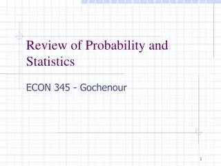
Probability and Statistics Review Thursday Mar 12
מודל למידה מה המשתנים החשובים? מה הטווח שלהם? מהן הקומבינציות החשובות?
חזרה מהירה על הסתברות • מאורע , אוסף מאורעות • משתנה מקרי • הסתברות מותנית , חוק ההסתברות השלמה , חוק השרשרת ,חוק בייס • תלות ואי תלות • שונות ,תוחלת ושונות משותפת • Moments
Sample space and Events • W : Sample Space, result of an experiment • If you toss a coin twice W = {HH,HT,TH,TT} • Event: a subset of W • First toss is head = {HH,HT} • S: event space, a set of events: • Closed under finite union and complements • Entails other binary operation: union, diff, etc. • Contains the empty event and W
Probability Measure • Defined over (W,S) s.t. • P(a) >= 0 for all a in S • P(W) = 1 • If a, b are disjoint, then • P(a U b) = p(a) + p(b) • We can deduce other axioms from the above ones • Ex: P(a U b) for non-disjoint event
Visualization • We can go on and define conditional probability, using the above visualization
הסתברות מותנית • P(F|H) = Fraction of worlds in which H is true that also have F true
Rule of total probability B2 B5 B3 B4 A B1 B7 B6
Bayes Rule • We know that P(smart) = .7 • If we also know that the students grade is A+, then how this affects our belief about his intelligence? • Where this comes from?
דוגמא במפעל פעולות שתי מכונות A ו-B . 10% מתוצרת המפעל מיוצרת במכונה A ו-90% במכונה B. 1% מהמוצרים המיוצרים במכונה A ו 5% מהמוצרים המיוצרים במכונה B הם פגומים. • נבחר מוצר אקראי, מה ההסתברות שהוא פגום? • נמצא מוצר שהוא פגום, מה ההסתברות שיוצר במכונה A? • אחרי ביקור של טכנאי שמטפל במכונה B , מוצאים ש 1.9% ממוצרי המפעל הם פגומים. מה עכשיו ההסתברות שמוצר המיוצר במכונה B יהיה פגום? פתרון: נגדיר את המאורעות הבאים: A-המוצר הנבחר יוצר במכונה A , B-המוצר הנבחר יוצר במכונה B, C-המוצר שנבחר פגום. א. עפ"י נוסחת ההסתברות השלמה מתקיים: P(C|A)*P(A)+P(C|B)*P(B) 0.046=0.01*0.1+ 0.05*0.9 ב. עפ"י נוסחת בייס:P(A|C)=P(C|A)*P(A)/P(C) => P(A|C)=0.01*0.1/0.046=0.021
משתנה מקרי בדיד • מ"מ הוא פונקציה ממרחב המאורעות הכללי (העולם) למרחב המאפיינים • בעצם ניתן לייצג התפלגות חדשה על פי המשתנה המקרי • Modeling students (Grade and Intelligence): • W = all possible students • What are events • Grade_A = all students with grade A • Grade_B = all students with grade A • Intelligence_High = … with high intelligence
Random Variables W I:Intelligence High low A A+ G:Grade B
Random Variables W I:Intelligence High low A A+ G:Grade B P(I = high) = P( {all students whose intelligence is high})
הסתברות משותפת • Joint probability distributions quantify this • P( X= x, Y= y) = P(x, y) • How probable is it to observe these two attributes together? • How can we manipulate Joint probability distributions? • דוגמא:מרכיבים באקראי מס' דו סיפרתי מהספרות 1,2,3,4. • יהי X מס' הספרות השונות המופיעות במס' ו Y מס' הפעמים שהספרה 1 מופיעה. • מהי ההתפלגות המשותפת של הזוג (X,Y)?
חוק השרשרת • Always true • P(x,y,z) = p(x) p(y|x) p(z|x, y) • = p(z) p(y|z) p(x|y, z) • =… • כדי לסבך קצת את העניינים נוסיף לשאלה מקודם • את הנתון הבא z יהיה מס הפעמים שמופיע ספרה גדולה ממש מ 2 • P(x=2,y=1,z=1)=P(x=2)*P(y=1|x=2)*P(z=1|y=1,x=2) • =0.75*[(6/16)/P(x=2)]*[(4/16)/(6/16)]
Conditional Probability events But we will always write it this way:
הסתברות השולית • We know P(X,Y), what is P(X=x)? • We can use the low of total probability, why? B2 B5 B3 B4 A B1 B7 B6
Marginalization Cont. • Another example
Bayes Rule cont. • You can condition on more variables
אי תלות • X is independent of Y means that knowing Y does not change our belief about X. • P(X|Y=y) = P(X) • P(X=x, Y=y) = P(X=x) P(Y=y) • Why this is true? • The above should hold for all x, y • It is symmetric and written as X Y
CI: Conditional Independence • X Y | Z if once Z is observed, knowing the value of Y does not change our belief about X • The following should hold for all x,y,z • P(X=x | Z=z, Y=y) = P(X=x | Z=z) • P(Y=y | Z=z, X=x) = P(Y=y | Z=z) • P(X=x, Y=y | Z=z) = P(X=x| Z=z) P(Y=y| Z=z) We call these factors : very useful concept !!
Properties of CI • Symmetry: • (X Y | Z) (Y X | Z) • Decomposition: • (X Y,W | Z) (X Y | Z) • Weak union: • (X Y,W | Z) (X Y | Z,W) • Contraction: • (X W | Y,Z) & (X Y | Z) (X Y,W | Z) • Intersection: • (X Y | W,Z) & (X W | Y,Z) (X Y,W | Z) • Only for positive distributions! • P()>0, 8, ;
Monty Hall Problem You're given the choice of three doors: Behind one door is a car; behind the others, goats. You pick a door, say No. 1 The host, who knows what's behind the doors, opens another door, say No. 3, which has a goat. Do you want to pick door No. 2 instead?
Monty Hall Problem: Bayes Rule : the car is behind door i, i = 1, 2, 3 : the host opens door j after you pick door i
Monty Hall Problem WLOG, i=1, j=3
Monty Hall Problem: Bayes Rule cont. • You should switch!
Moments Mean (Expectation): Discrete RVs: Continuous RVs: Variance: Discrete RVs: Continuous RVs:
Properties of Moments Mean If X and Y are independent, Variance If X and Y are independent,
The Big Picture Probability Model Data Estimation/learning
Statistical Inference • Given observations from a model • What (conditional) independence assumptions hold? • Structure learning • If you know the family of the model (ex, multinomial), What are the value of the parameters: MLE, Bayesian estimation. • Parameter learning
MLE • Maximum Likelihood estimation • Example on board • Given N coin tosses, what is the coin bias (q )? • Sufficient Statistics: SS • Useful concept that we will make use later • In solving the above estimation problem, we only cared about Nh, Nt , these are called the SS of this model. • All coin tosses that have the same SS will result in the same value of q • Why this is useful?
Statistical Inference We need some concepts from information theory • Given observation from a model • What (conditional) independence assumptions holds? • Structure learning • If you know the family of the model (ex, multinomial), What are the value of the parameters: MLE, Bayesian estimation. • Parameter learning
Information Theory • P(X) encodes our uncertainty about X • Some variables are more uncertain that others • How can we quantify this intuition? • Entropy: average number of bits required to encode X P(Y) P(X) X Y
Information Theory cont. • Entropy: average number of bits required to encode X • We can define conditional entropy similarly • We can also define chain rule for entropies (not surprising)
Mutual Information: MI • Remember independence? • If XY then knowing Y won’t change our belief about X • Mutual information can help quantify this! (not the only way though) • MI: • Symmetric • I(X;Y) = 0 iff, X and Y are independent!
Continuous Random Variables What if X is continuous? Probability density function (pdf) instead of probability mass function (pmf) A pdf is any function that describes the probability density in terms of the input variable x.
PDF Properties of pdf Actual probability can be obtained by taking the integral of pdf E.g. the probability of X being between 0 and 1 is
Cumulative Distribution Function Discrete RVs Continuous RVs
Acknowledgment Andrew Moore Tutorial:http://www.autonlab.org/tutorials/prob.html Monty hall problem: http://en.wikipedia.org/wiki/Monty_Hall_problem http://www.cs.cmu.edu/~guestrin/Class/10701-F07/recitation_schedule.html