Download
1 / 26
260 likes | 363 Views
Improving Probabilistic Ensemble Forecasts of Convection through the Application of QPF-POP Relationships. Christopher J. Schaffer 1 William A. Gallus Jr. 2 Moti Segal 2 1 National Weather Service, WFO Goodland 2 Iowa State University, Ames, IA. Ensemble vs. Deterministic.

E N D
Improving Probabilistic Ensemble Forecasts of Convection through the Application of QPF-POP Relationships Christopher J. Schaffer1 William A. Gallus Jr.2 Moti Segal2 1 National Weather Service, WFO Goodland 2 Iowa State University, Ames, IA
Ensemble vs. Deterministic • Probabilistic forecasts provide uncertainty • Small errors in forecast’s initial conditions grow exponentially (Hamill and Colucci 1997) • Ensemble mean forecasts tend to be more skillful (Smith and Mullen 1993, Ebert 2001, Chakraborty and Krishnamurti 2006)
Gallus and Segal (2004) and Gallus et al. (2007) • Precipitation-binning technique for deterministic forecasts • Larger forecasted precipitation => greater probability to receive precipitation • POPs increased further if different models showed an intersection of grid points with rain in a bin
Overview of study Goals • Apply post-processing techniques similar to the Gallus and Segal (2004) technique to ensemble forecasts • Examine how the forecasts compare to those from more traditional approaches
Data • NOAA Hazardous Weather Testbed (HWT) Spring Experiments (2007 and 2008) • Ensemble of ten WRF-ARW members with 4 km grid spacing run by Center for Analysis and Prediction of Storms (CAPS) • 30 hours per case (five 6-hour time periods); 00Z • Present study uses a subdomain of 2007/2008 • Coarsened onto 20 km grid spacing
Subdomain of Present Study 1980 km x 1840 km rather than 3000 km x 2500 km (2007)
Methodology • Creation of 2D POP tables • Forecasted precipitation amount within a bin • Maximum or average amount • Number of ensemble members forecasting agreement on precipitation amounts above a threshold
Methodology continued • Seven precipitation bins • POPs assigned through hit rates • NCEP Stage IV observations designated hits • Three thresholds: 0.01, 0.10, and 0.25 inch -h is the number of “hits”, or points where the observed precipitation also exceeded the specified threshold -f is the number of grid points with precipitation forecasted for a given bin/member scenario
Approach #1 Two-parameter point forecast approach
Max_thr POPs for April 23, 2007 06Z – 12Z
Cali_trad POPs for April 23, 2007 06Z – 12Z
Approach #2 Two-parameter neighborhood approach
Two-parameter neighborhood approach • Neighborhoods: Theis et al. (2005), Ebert (2009) • Within a specified square area around a center point, the max or aveprecip. amount is determined and binned • Number of points within the neighborhood that have forecast precip. amounts greater than a threshold • Spatially generated ensemble • Forecasts for each member 3x3 Neighborhood
Scatterplot of Brier scores (0.01 inch threshold)
Scatterplot of Brier scores (0.10 and 0.25 inch thresholds)
Approach #3 Combination of methods
Combination of methods • Considers each method as an ensemble member that itself consists of ensemble members • Uses the different POP tables to determine POPs for each method, then averages POPs • Different trends in POP fields • Many variations of the approach
Conclusions • Two-parameter point forecast approach • Improvements over Cali_trad, which encouraged the development of other approaches • Two-parameter neighborhood approach • Deterministic, but comparable to Cali_trad • Improvements due to spatial ensembles • Increased neighborhood size led to better Brier scores • Combination approach • Brings several methods/approaches together by averaging POPs • Statistically significantly different Brier scores compared to Cali_trad at 90% C.I.
This research was funded in part by National Science Foundation grants ATM-0537043 and ATM-0848200, with funds from the American Recovery and Reinvestment Act of 2009. christopher.schaffer@noaa.gov