Download
1 / 9
110 likes | 270 Views
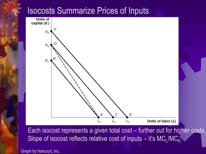
Isocosts Summarize Prices of Inputs. Each isocost represents a given total cost – further out for higher costs. Slope of isocost reflects relative cost of inputs – it’s MC L /MC K. Graph by Harcourt, Inc. Isoquants Summarize Technology.

E N D
Isocosts Summarize Prices of Inputs Each isocost represents a given total cost – further out for higher costs. Slope of isocost reflects relative cost of inputs – it’s MCL/MCK Graph by Harcourt, Inc.
Isoquants Summarize Technology Each isoquant represents a quantity of output – further out for more. Slope of isoquant is the marginal rate of technical substitution. MRTS = MPL/MPK Graph by Harcourt, Inc.
Perfect Technological Complements No substitution is possible, so isoquants are right angles. Note that perfect substitutes would be straight lines - look like isocosts. Graph by Harcourt, Inc.
Profit Maximizing Choice of Inputs For the desired quantity of output, set MCL/MCK = MPL/MPK so the last dollar spent on each input is equally productive. Graph by Harcourt, Inc.
Long Run Effect of an Increase in the Wage A wage increase implies higher MC and thus lower optimal output. With the lower output (scale effect) reduce labor (Y) but steeper isoquant (substitution effect) so increase capital (Z). Graph by Harcourt, Inc.
Categories of Demand Elasticities Vertical ED is perfectly inelastic. Horizontal ED is perfectly elastic. Curved ED is unit elastic. At their intersection, both demand curves are unit elastic, but the steeper one is relatively less elastic overall. Graph by Harcourt, Inc.
Elasticities Along a Straight-line Demand Curve Unit elastic at midpoint. Elastic over top half. Inelastic over bottom half. Note that total wage bill is maximized at point of unit elasticity. Graph by Harcourt, Inc.
Firm-Specific Training MRP > W Without training MRP0. With training is MRP1 first then MRP2. To share cost, firm can pay W3 and not lose worker, who is only worth W0 to other firms. If product demand, and thus MRP drops, W3 will likely still be below the new MRP and thus the worker will not be laid off. Graph by Harcourt, Inc.
Path of Employment with Adjustment Costs Costs of hiring (H) and firing (F) make it optimal to have less employment during a boom and more employment during a bust. Only hire if MRP-W>H, only fire if W-MRP>F.