Lecture 4: Models of Price Competition

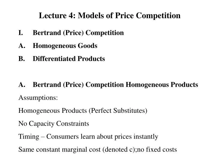
1. Lecture 4:Models of Price Competition • Bertrand (Price) Competition • A. Homogeneous Goods • B. Differentiated Products • Bertrand (Price) Competition Homogeneous Products • Assumptions: • Homogeneous Products (Perfect Substitutes) • No Capacity Constraints • Timing – Consumers learn about prices instantly • Same constant marginal cost (denoted c);no fixed costs

2. Di(pi) if pi<pj Di(pi,pj) = .5 Di (pi) if pi=pj 0 if pi>pj Firms choose prices simultaneously and non-cooperatively. NE is a pair of prices pi*,pj* such that: pi(pi*,pj*)  pi(pi,pj*) for all pi pj(pi*,pj*)  pj(pi*,pj) for all pj Claim: pi*=c, pj*=c Result is referred to as the Bertand Paradox – It takes only two firms to obtain (perfect) competition.

3. B1. Bertrand (Price) Competition: Differentiated Products Example: q1=90-2p1+p2, q2=90-2p2+p1, No variable costs p1= p1q1 = p1(90-2p1+p2) =90p1 – 2p12 + p2p1 dp1/dp1=90-4p1+p2 =0 or p1=(90+p2)/4 (Reaction function of firm 1) Similarly, p2=(90+p1)/4 (Reaction function of firm 2)

4. Reaction function of firm 1 p2 Reaction function of firm 2 p1 Equilibrium p1*=p2*=30 p1= p1q1 = p1(90-2p1+p2)= 30(60)=1800 p2= p2q2 = p2(90-2p2+p1)= 30(60)=1800 No Bertand Paradox with Differentiated Products

5. Comparison between Bertrand and Cournot Competition: Example: q1=90-2p1+p2, q2=90-2p2+p1 Bertrand Competition: p1*=p2*=30, q1*=q2*=60, p1 =p2 = 1800 Cournot Competition: Derive (inverse) demand curves: p1=(270-2q1-q2)/3, p2=(270-2q2-q1)/3 p1= p1q1 = (270-2q1-q2)q1/3. FOC: 270-4q1-q2=0. q1*=q2*=54, p1*=p2*=36, p1 =p2 =1944

6. Intuitively Explaining the Results Under Bertrand Competition, the elasticity of demand is e(B)=-(P/Q) (dQ/dP) = 2P/Q e(C)=-(P/Q) (dQ/dP) = 1.5P/Q Perceived Elasticity of Demand Lower Under Cournot Competition. (True for all linear demand curves.) Hence, profits are higher under Cournot competition.

7. B A 0 1 B2: Price Competition with Differentiated Products: Hotelling (1929) Model City of length one (1) unit Two firms: denoted A & B at different ends of the interval Consumers uniformly distributed on [0,1]. (Another interpretation is that consumer tastes are uniformly distributed on the interval) Unit Cost is “c” Transportation cost of “k” per unit distance (x) Consumers have unit demands, i.e., they purchase one unit of good Except for distance, goods are homogenous with gross utility “v.”

8. B A 0 1 x A consumer located at “x” incurs a transportation cost of “kx” to purchase from firm A, and a transportation cost of “k(1-x)” to purchase from firm B. Net utility: U(A)=v-pA-kx (where price pA is charged by firm A) Net utility: U(B)=v-pB-k(1-x) (where price pB is charged by firm B) Under the assumption that prices are not too high relative to “v,” the market is fully covered. In such a case, marginal consumer (x) is indifferent between the two good, i.e., U(A)=U(B). Marginal consumer x=(pB – pA + k)/2k.

9. Demand for good A, DA(pA,pB)= x= (pB – pA + k)/2k. Demand for good B, DB(pA,pB)= (1-x) =(pA – pB + k)/2k. Hence: A= (pA-c) DA(pA,pB)= (pA-c)(pB – pA + k)/2k. B= (pB-c) DB(pA,pB)= (pB-c)(pA – pB + k)/2k. FOC: - (pA-c) + (pB – pA + k) = 0 pA=(pB + c + k)/2. (firm A) - (pB-c) + (pA – pB + k) = 0 pB=(pA + c + k)/2. (firm B) Nash equilibrium prices: pA*=pB*= c+k. Equilibrium profits: A*= B*= k/2. When the products are more differentiated (larger k), prices are higher. When k 0, the model approaches Bertrand competition with homogeneous products.

10. B A 0 4 8 9 x 4-x • Different Locations along line: • We looked at the case of maximum differentiation. • When the products are in the same location, competition will force the price down to marginal cost (pA*=pB*= c). • Different Locations (but not at the end of the line) - need quadratic transportation costs to insure equilibrium: Example PS2, #4 U(A)=v-pA-2x2 , U(B)=v-pB-2(4-x)2 x=(pB-pA+32)/16 A= (pA-c) (4+x) , B= (pB-c) [1+(4-x)]