Download
1 / 22
220 likes | 229 Views
1. 2. 3. 4. 5. 6. n. 1. 1. 2. 2. 3. 3. 4. 4. 5. 5. 6. 6. n. n. Transport Calculations. Advection. Dispersion. Reaction. ADVECTION. Cells are numbered from 1 to N.

E N D
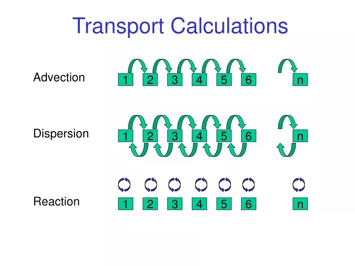
1 2 3 4 5 6 n 1 1 2 2 3 3 4 4 5 5 6 6 n n Transport Calculations Advection Dispersion Reaction
ADVECTION • Cells are numbered from 1 to N. • Index numbers (of SOLUTION, EQUILIBRIUM_PHASES, etc) are used to define the solution and reactants in each cell • SOLUTION 0 (or N+1) enters the column • Water is “shifted” from one cell to the next
ADVECTION • TRANSPORT adds dispersion, stagnant zones, and heat transport
ADVECTION • Number of cells • Number of shifts • If kinetics—time step
ADVECTION • Output file • Cells to print • Shifts to print • Selected-output file • Cells to print • Shifts to print
T.1. Exercise • Run the Oklahoma simulation in a 10-cell column. a. Change the log K to –15 for the following two surface complexation reactions: Hfo_wOH + Mg+2 = Hfo_wOMg+ + H+ Hfo_wOH + Ca+2 = Hfo_wOCa+ + H+ b. Initial conditions: equilibrate the following brine with calcite and dolomite.
T.1. Exercise (continued) c. Initial conditions: Equilibrate 1 mol of exchanger with the reacted brine and place in each cell of the column. d. Initial conditions: Equilibrate 0.07 mol of surface complexation sites with the reacted brine. Assume 600 m^2/g specific surface area and 30 grams of sorbing material. Place the surface in each cell of the column. e. Define evaporated rainwater with the following composition:
T.1. Exercise (continued) f. Assume the rainwater reacts with calcite and dolomite in the soil zone and the soil zone pCO2 = 10^-1.5. This water flows into the column. g. Replace half the pore volume of the column with the infilling water. h. Plot pH, Cl (mol/kgw) and total dissolved As (ug/kgw) versus cell number.
T.2. Questions • Describe the Cl- profile in the column at the end of the simulation. • Describe the pH profile in the column at the end of the simulation. • What is the pH at which arsenic appears to become a problem?
TRANSPORT • Cell lengths Velocity=length/time step! • Dispersivities
TRANSPORT • Boundary conditions • Flow direction • Diffusion coefficient • Heat
TRANSPORT • Stagnant cells/dual porosity -One stagnant cell -Multiple stagnant cells
PHAST • 3D Flow model • PHREEQC chemistry • Capabilities • Specified, leaky, flux boundary conditions • Water table/confined • Wells • Rivers • Sequential iteration • Transport all elements conservatively • Run reactions in each cell • Repeat
PHAST • All the data for flow model—porosity, hydraulic conductivity • All the data for solute transport model—dispersivity, boundary conditions • All the data for chemistry • Apply initial conditions by index numbers of PHREEQC • Associate solutions by index numbers for boundary conditions
PHAST • Flow and transport file • Keyword driven input • Same input style as PHREEQC • Chemistry data file • Exactly a PHREEQC input file
FLOW ANDTRANSPORT DATA FILE GRID -uniform x 0 90000 16 -uniform y 0 48000 9 -uniform z 0 400 5 MEDIA -zone 0. 0. 0. 90000. 48000. 400. -porosity 0.22 -long_dispersivity 4000. -trans_dispersivity 50. -Kx 1.373e-5 -Ky 1.373e-5 -Kz 1.373e-7 -storage 0
FLOW-AND-TRANSPORT DATA FILE FLUX_BC -zone 30000. 3000. 400. 90000. 45000. 400. -flux -10e-5 -associated_solution 1 SPECIFIED_VALUE_BC # Lake Stanley Draper -zone 30000. 14000 300. 32000. 20000. 400. -head 348. -associated_solution 1 LEAKY_BC -zone 0. 48000. 0. 29000. 48000. 400. -hydraulic 1.618e-5 -thickness 30000. -head 305.0 -associated 1 CHEMISTRY_IC -zone 0. 0. 0. 90000. 48000. 400. -solution 2 -equilibrium_phases 2 -exchange 2 -surface 2
MODELVIEWER • Solid/None • Model features • Grid lines • Color bar • Show—select items to be present in the visualization
MODELVIEWER • Data • Color bar • Geometry • Model features • Crop • Animation • Tools—select menus by which you can change the look of the features selected by Show.
Buttons • Left mouse—3D rotate • Shift Left mouse—2D rotate in plane of screen • Middle mouse—Drag • Right mouse—Grow and shrink
T.2. Exercise • Run phast from a command prompt in the directory Friday\phast.ok phast ok • Start ModelViewer • File->Open Friday\phast.ok\ok.mv • Use ModelViewer to make an animation of the evolution of arsenic in ground-water chemistry in Central Oklahoma