Interpreting Bi-variate OLS Regression

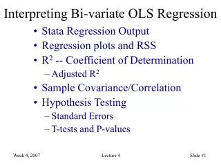
Interpreting Bi-variate OLS Regression • Stata Regression Output • Regression plots and RSS • R2 -- Coefficient of Determination • Adjusted R2 • Sample Covariance/Correlation • Hypothesis Testing • Standard Errors • T-tests and P-values

Stata Regression Model: Regressing Political Ideology Scale onto “Militant” Y average of variables 81 and 82 (reversed), 84, 85 and 86 X is variable 98: Political Ideology 1 = “strong Lib” 7=“strong Cons”

Regression Output regress militant p98_ideo, beta

Regression Descriptive Statistics corr militant p98_ideo, means

Regression Plot

Measuring “Goodness of Fit” • Root of Mean Squared Error (“Root MSE”) • Measures spread around the regression line • Coefficient of Determination (R2) “model” or explained sum of squares “total” sum of squares

unexplained deviation explained deviation Explaining R2 For each observation Yi, variation around the mean can be decomposed into that which is “explained” by the regression and that which is not: Book terminology: TSS = (all)2 RSS = (unexplained)2 ESS = (explained)2 Stata terminology: Residual = (unexplained)2 Model = (explained)2 Total = (all)2

Sample Covariance & Correlation • Sample covariance for a bivariate model is defined as: • Sample correlations (r) “standardize” covariance by dividing by the product of the X and Y standard deviations: Sample correlations range from -1 (perfect negative relationship) to +1 (perfect positive relationship)

Standardized Regression Coefficients(aka “Beta Weights” or “Betas”) • Formula: • In our example: • Interpretation: the number of std. deviations change in Y one should expect from a one-std. deviation Change in X.

Hypothesis Tests for Regression Coefficients • For our model: Yi = 2.289+0.365*Xi+ei • Another sample of 2584 observations would lead to different estimates for b0 and b1. If we drew many such samples, we’d get the sample distribution of the estimates • We need to estimate the sample distribution, (because we usually can’t see it) based on our sample size and variance

To do that we calculate SEbs (Bivariate case only)

For our model: b0 = 2.289, and SEb0 = 0.055 b1 = 0.365, and SEb1 = 0.012 Interpreting Standard Errors Assuming that we estimated the sample standard error correctly, we can identify how many standard errors our estimate is away from zero. The T-test reports the number of standard errors our estimate falls away from zero. Thus, the “T” for b1 is 30.24 for our model. (rounding!) Estimated Sampling Distribution for b1 0 (which is 30.24 SEb1 “units” away from b1) b1 = 0.365 b1 - SEb1= 0.353 b1 + SEb1= 0.373

Classical Hypothesis Testing • Assume that b1 is zero. What is the probability that your sample would have • resulted in an estimate for b1 that is 30.24 SEb1’s away from zero? • To find out, determine the cumulative density of the estimated sampling • distribution that falls more than 30.24 SEb1’s away from zero. • See Table A4.1, page 350, in Hamilton. It reports discrete “p-values”, given • the sample size and t-values. Note the distinction between 1 and 2 sided tests • In general, if the t-stat is above 2, • the p-value will be <0.05 -- which is • the acceptable upper limit in a • classical hypothesis test. Note: in Stata-speak, a p-value is a “p>|t|” Assume that b1 = 0.0 (null hypothesis) Estimated b1 = 0.365 (working hypothesis)

Coming up... • For Tuesday • Use variables 87-89 to make an “egalitarian” index for your dependent variable (Y) • Use p98_ideo (ideology) as the independent variable (X) to predict egaitarianism. Fully interpret the results. • Walk through the entire interpretation • Build a Stata do-file as you go • For Next Week: • Remainder of Chapter 2 • Schedule: • Feb 21: Residual Analysis & Exam Review • Feb 28: Exam

Interpreting Bi-variate OLS Regression