Download
1 / 17
290 likes | 664 Views
The Vector Field Histogram. Erick Tryzelaar November 14, 2001 Robotic Motion Planning A Method Developed by J. Borenstein and Y. Koren. The Problem. To simultaneously: Detect, and avoid, unknown obstacles in real-time Steer in the best direction that leads to some target, k targ

E N D
The Vector Field Histogram Erick Tryzelaar November 14, 2001 Robotic Motion Planning A Method Developed by J. Borenstein and Y. Koren
The Problem • To simultaneously: • Detect, and avoid, unknown obstacles in real-time • Steer in the best direction that leads to some target, ktarg • Do it as quickly as possible 24-700 Robotic Motion Planning
The Solution: The Vector Field Histogram (VFH) • The first step generates a 2D Cartesian coordinate from each range sensor, and increments that position in the histogram gridC Note: this method does not depend on a specific sensor model 24-700 Robotic Motion Planning
The Solution, Continued (2) • The next step filters this two dimensional grid down into a one dimensional structure • The final step calculates the steering angle and the velocity controls from this structure 24-700 Robotic Motion Planning
First, Some Terminology • VCP • The center point of the robot • Obstacle vector • A vector pointing from a cell in C* to the VCP Robot VCP 24-700 Robotic Motion Planning
Step 2: Mapping 2D onto 1D • In order to simplify calculations, the 2D grid used in this step is a window of C, with constant dimensions, and centered on the VCP, called the active grid, or C*. 24-700 Robotic Motion Planning
Step 2: Continued (2) • This is then mapped onto a 1D structure known as a polarhistogram, or H. A polar histogram is a one-dimensional grid comprising of n angular sections with width a Figure included with permission from J. Borenstein 24-700 Robotic Motion Planning
Step 2: Continued (3) • In order to generate H, we must first map every cell in C* onto a 1D point in H’s coordinate system 24-700 Robotic Motion Planning
Step 2: Continued (4) Figure included with permission from J. Borenstein 24-700 Robotic Motion Planning
Step 2: Continued (5) • Because H at this point contains discrete points, a smoothing function can be applied in order to better approximate the environment 24-700 Robotic Motion Planning
Step 3: Computing the Steering Direction • A typical polar histogram contains “peaks”, or sectors with a high polar obstacle density (POD), and “valleys”, sectors that contain low POD’s • A valley below some threshold is called a candidate valley Figure included with permission from J. Borenstein 24-700 Robotic Motion Planning
Step 3: Continued (2) • From all the candidate valleys, the valley closest to the ktarg is selected • The type of the valley is dependant on the some consecutive number of sectors, Smax, under the threshold • Wide is greater than Smax • Narrow is less than Smax 24-700 Robotic Motion Planning
Step 3: Continued (3) • In that valley, kn is selected from the first or the last sector, whichever is closer to ktarg • Wide valleys: kf = kn ± Smax, which results in kf in the valley • Narrow valleys: kf is the last sector in the valley • Then q = (kn + kf)/2 24-700 Robotic Motion Planning
Step 3: Selecting the Threshold • If set too high, the robot may be too close to an obstacle, and moving too quickly in order to prevent a collision • However, if set too low, VFH can miss some valid candidate valleys • Generally, the threshold does not need much tuning, unless the application of the robot requires very fast navigation of tightly packed obstacles 24-700 Robotic Motion Planning
Step 3: Speed Controls 24-700 Robotic Motion Planning
Comparison to Potential Fields • Influences of a bad sensor read is minimized because it is averaged out with prior data • Instability in traveling down a narrow corridor is eliminated because the polar histogram varies only slightly between sonar reads • The “repulsive forces” from obstacles cannot counterbalance the “attractive force” from the target and trap the robot in a local minima, as VFH only tries to drive through the best possible valley, regardless if it leads away from the target 24-700 Robotic Motion Planning
Comparison, Continued (2) • However, VFH can not solve all the limitations inherent with the potential field method • Nothing prevents the robot from being caught in a real local minima, or a cycle • When this occurs, a global path planner must be used to generate intermediary targets for the VFH until it is out of the trap Robot ktarg 24-700 Robotic Motion Planning