Download
1 / 24
240 likes | 322 Views
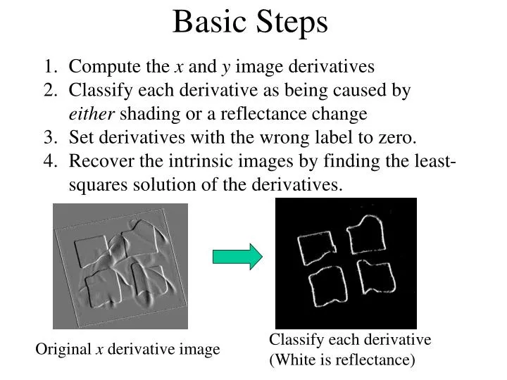
Basic Steps. Compute the x and y image derivatives Classify each derivative as being caused by either shading or a reflectance change Set derivatives with the wrong label to zero. Recover the intrinsic images by finding the least-squares solution of the derivatives.

E N D
Basic Steps • Compute the x and y image derivatives • Classify each derivative as being caused by either shading or a reflectance change • Set derivatives with the wrong label to zero. • Recover the intrinsic images by finding the least-squares solution of the derivatives. Classify each derivative (White is reflectance) Original x derivative image
Learning the Classifiers • Combine multiple classifiers into a strong classifier using AdaBoost (Freund and Schapire) • Choose weak classifiers greedily similar to (Tieu and Viola 2000) • Train on synthetic images • Assume the light direction is from the right Shading Training Set Reflectance Change Training Set
Results without considering gray-scale Using Both Color and Gray-Scale Information
Reflectance Shading Some Areas of the Image Are Locally Ambiguous Is the change here better explained as Input ? or
Propagating Information • Can disambiguate areas by propagating information from reliable areas of the image into ambiguous areas of the image
Propagating Information • Consider relationship between neighboring derivatives • Use Generalized Belief Propagation to infer labels
Setting Compatibilities • Set compatibilities according to image contours • All derivatives along a contour should have the same label • Derivatives along an image contour strongly influence each other β= 0.5 1.0
Improvements Using Propagation Input Image Reflectance Image Without Propagation Reflectance Image With Propagation
(More Results) Reflectance Image Input Image Shading Image
Summary Belief propagation is a feasible way to do inference in some Markov Random Fields. We showed applications of this approach to a number of low-level vision problems, including super-resolution, motion, and shading/reflectance discrimination. next talk: presentations/bengaluruDeblur.ppt or keynote:presentations/motioninvVenice.key
Inference in Markov Random Fields Gibbs sampling, simulated annealing Iterated conditional modes (ICM) Belief propagation Application examples: super-resolution motion analysis shading/reflectance separation Graph cuts Variational methods
Gibbs Sampling and Simulated Annealing • Gibbs sampling: • A way to generate random samples from a (potentially very complicated) probability distribution. • Fix all dimensions except one. Draw from the resulting 1-d conditional distribution. Repeat for all dimensions, and repeat many times • Simulated annealing: • A schedule for modifying the probability distribution so that, at “zero temperature”, you draw samples only from the MAP solution. Reference: Geman and Geman, IEEE PAMI 1984.
3. Sampling draw a ~ U(0,1); for k = 1 to n if break; ; Sampling from a 1-d function • Discretize the density function 2. Compute distribution function from density function
x2 x1 Gibbs Sampling Slide by Ce Liu
Gibbs sampling and simulated annealing Simulated annealing as you gradually lower the “temperature” of the probability distribution ultimately giving zero probability to all but the MAP estimate. What’s good about it: finds global MAP solution. What’s bad about it: takes forever. Gibbs sampling is in the inner loop…
Gibbs sampling and simulated annealing So you can find the mean value (MMSE estimate) of a variable by doing Gibbs sampling and averaging over the values that come out of your sampler. You can find the MAP value of a variable by doing Gibbs sampling and gradually lowering the temperature parameter to zero.
Inference in Markov Random Fields Gibbs sampling, simulated annealing Iterated conditional modes (ICM) Belief propagation Application examples: super-resolution motion analysis shading/reflectance separation Graph cuts Variational methods
Iterated conditional modes • For each node: • Condition on all the neighbors • Find the mode • Repeat. • Compare with Gibbs sampling… • Very small region over which it’s a local maximum Described in: Winkler, 1995. Introduced by Besag in 1986.
i Region marginal probabilities i j
Belief propagation equations Belief propagation equations come from the marginalization constraints. i i j = i j i