Download
1 / 51
510 likes | 530 Views
Chapter 2 EVAPORATION. Content. Type of Evaporation equipment and Methods Overall Heat Transfer Coefficient in Evaporators Calculation Methods for Single Effect Evaporators Calculation Methods for Multiple Effects Evaporators Condenser for Evaporator Evaporation using Vapor Recompression.

E N D
Content • Type of Evaporation equipment and Methods • Overall Heat Transfer Coefficient in Evaporators • Calculation Methods for Single Effect Evaporators • Calculation Methods for Multiple Effects Evaporators • Condenser for Evaporator • Evaporation using Vapor Recompression
Evaporation • Heat is added to a solution to vaporize the solvent, which is usually water. • Case of heat transfer to a boiling liquid. • Vapor from a boiling liquid solution is removed and a more concentrated solution remains. • Refers to the removal of water from an aqueous solution. • Example: concentration of aqueous solutions of sugar. In these cases the crystal is the desired product and the evaporated water is discarded.
Pressure and temperature Materials of construction Foaming or frothing Scale deposition Processing Factors solubility Temperature sensitivity of materials Concentration in the liquid
Processing Factors • Concentration dilute feed, viscosity , heat transfer coefficient, h concentrated solution/products, , and h . • Solubility concentration , solubility , crystal formed. solubility with temperature . • Temperature. heat sensitive material degrade at higher temperature & prolonged heating.
Foaming/frothing. caustic solutions, food solutions, fatty acid solutions form foam/froth during boiling. entrainment loss as foam accompany vapor. • Pressure and Temperature pressure , boiling point . concentration , boiling point. heat-sensitive material operate under vacuum. • Material of construction minimize corrosion.
Effect of Processing Variables on Evaporator Operation. • TF TF < Tbp, some of latent heat of steam will be used to heat up the cold feed, only the rest of the latent heat of steam will be used to vaporize the feed. Is the feed is under pressure & TF > Tbp, additional vaporization obtained by flashing of feed. • P1 desirable T [Q = UA(TS – T1)], A & cost . T1 depends on P1 will T1.
PS PS will TS but high-pressure is costly. optimum TS by overall economic balances. • BPR The concentration of the solution are high enough so that the cPand Tbp are quite different from water. BPR can be predict from Duhring chart for each solution such as NaOH and sugar solution. • Enthalpy–concentration of solution. for large heat of solution of the aqueous solution. to get values for hF and hL.
vapor,V to condenser T1 , yV , HV feed, F TF , xF , hF. heat-exchanger tubes P1 T1 steam, S TS , HS condensate, S TS , hS concentrated liquid, L T1 , xL , hL Simplified Diagram of single-effect evaporator
Single-effect evaporators; • the feed (usually dilute) enters at TF and saturated steam at TSenters the heat-exchange section. • condensed leaves as condensate or drips. • the solution in the evaporator is assumed to be completely mixed and have the same composition at T1. • the pressure is P1, which is the vapor pressure of the solution at T1. • wasteful of energy since the latent heat of the vapor leaving is not used but is discarded. • are often used when the required capacity of operation is relatively small, but it will wasteful of steam cost.
Calculation Methods for Single-effect Evaporator. • Objectives: to calculate - vapor, V and liquid, L flowrates. - heat transfer area, A - overall heat-transfer coefficient, U. - Fraction of solid content, xL. • To calculate V & L and xL, - solve simultaneously total material balance & solute/solid balance. F = L + V total material balance F (xF) = L (xL) solute/solid balance
To calculate A or U, - no boiling point rise and negligible heat of solution: calculate hF, hL, Hv and . where, = (HS – Hs) h = cP(T – Tref) where, Tref = T1 = (as datum) cPF = heat capacity (dilute as water) HV= latent heat at T1 solve for S: F hF + S = L hL + V HV solve for A and U: q = S = U A T = UA (TS – T1)
To get BPR and the heat of solution: - calculate T1 = Tsat + BPR - get hFand hL from Figure 8.4-3. - get S & HVfrom steam tables for superheated vapor or HV = Hsat + 1.884 (BPR) - solve for S: F hF + S = L hL + V HV - solve for A and U: q = S = U A T = UA (TS – T1)
Example 8.4-1: Heat-Transfer Area in Single-Effect Evaporator. A continuous single-effect evaporator concentrates 9072 kg/h of a 1.0 wt % salt solution entering at 311.0 K (37.8 ºC) to a final concentration of 1.5 wt %. The vapor space of the evaporator is at 101.325 kPa (1.0 atm abs) and the steam supplied is saturated at 143.3 kPa. The overall coefficient U = 1704 W/m2 .K. calculate the amounts of vapor and liquid product and the heat-transfer area required. Assumed that, since it its dilute, the solution has the same boiling point as water.
V = ? T1 , yV , HV F = 9072 kg/h TF = 311 K xF = 0.01 hF. P1 = 101.325 kPa U = 1704 W/m2 T1 A = ? S , TS , HS PS = 143.3 kPa S, TS , hS L = ? T1 , hL xL = 0.015 Figure 8.4-1: Flow Diagram for Example 8.4-1
Solution; Refer to Fig. 8.4-1 for flow diagram for this solution. For the total balance, F = L + V 9072 = L + V For the balance on the solute alone, F xF = L xL 9072 (0.01) = L (0.015) L = 6048 kg/h of liquid Substituting into total balance and solving, V = 3024 kg/h of vapor
Since we assumed the solution is dilute as water; cpF = 4.14 kJ/kg. K (Table A.2-5) From steam table, (A.2-9) At P1 = 101.325 kPa, T1 = 373.2 K (100 ºC). HV = 2257 kJ/kg. At PS = 143.3 kPa, TS = 383.2 K (110 ºC). = 2230 kJ/kg. The enthalpy of the feed can be calculated from, hF = cpF (TF – T1) hF = 4.14 (311.0 – 372.2) = -257.508 kJ/kg.
Substituting into heat balance equation; F hF + S = L hL + V HV with hL = 0, since it is at datum of 373.2 K. 9072 (-257.508) + S (2230) = 6048 (0) + 3024 (2257) S = 4108 kg steam /h The heat q transferred through the heating surface area, A is q = S () q = 4108 (2230) (1000 / 3600) = 2 544 000 W Solving for capacity single-effect evaporator equation; q = U A T = U A (TS – T1) 2 544 000 = 1704 A (383.2 – 373.2) Solving, A = 149.3 m2.
Example 8.4-3: Evaporation of an NaOH Solution. An evaporator is used to concentrate 4536 kg/h of a 20 % solution of NaOH in water entering at 60 ºC to a product of 50 % solid. The pressure of the saturated steam used is 172.4 kPa and the pressure in the vapor space of the evaporator is 11.7 kPa. The overall heat-transfer coefficient is 1560 W/m2.K. calculate the steam used, the steam economy in kg vaporized/kg steam used, and the heating surface area in m2.
V, T1 , yV , HV F = 4536 kg/h TF = 60 ºC xF = 0.2 hF. P1 = 11.7 kPa U = 1560 W/m2 T1 A = ? S = ? TS , HS PS = 172.4 kPa S, TS , hS L, T1 , hL xL = 0.5 Figure 8.4-4: Flow Diagram for Example 8.4-3
Solution, Refer to Fig. 8.4-4, for flow diagram for this solution. For the total balance, F = 4536 = L + V For the balance on the solute alone, F xF = L xL 4536 (0.2) = L (0.5) L = 1814 kg/h of liquid Substituting into total balance and solving, V = 2722 kg/h of vapor
To determine T1 = Tsat + BPRof the 50 % concentrate product, first we obtain Tsat of pure water from steam table. At 11.7 kPa, Tsat = 48.9 ºC. From Duhring chart (Fig. 8.4-2), for a Tsat = 48.9 ºC and 50 % NaOH , the boiling point of the solution is T1 = 89.5 ºC. hence, BPR = T1 - Tsat = 89.5-48.9 = 40.6 ºC From the enthalpy-concentration chart (Fig.8.4-3), for TF = 60 ºC and xF = 0.2 get hF = 214 kJ/kg. T1 = 89.5 ºC and xL = 0.5 get hL = 505 kJ/kg.
For saturated steam at 172.4 kPa, from steam table, we get TS = 115.6 ºC and = 2214 kJ/kg. To get HV for superheated vapor, first we obtain the enthalpy at Tsat = 48.9 ºC and P1 = 11.7 kPa, get Hsat = 2590 kJ/kg. Then using heat capacity of 1.884 kJ/kg.K for superheated steam. So HV = Hsat + cP BPR = 2590 + 1.884 (40.6) = 2667 kJ/kg. Substituting into heat balance equation and solving for S, F hF + S = L hL + V HV 4535 (214) + S (2214) = 1814 (505) + 2722 (2667) S = 3255 kg steam /h.
The heat q transferred through the heating surface area, A is q = S () q = 3255 (2214) (1000 / 3600) = 2 002 000 W Solving for capacity single-effect evaporator equation; q = U A T = U A (TS – T1) 2 002 000 = 1560 A (115.6 – 89.5) Solving, A = 49.2 m2. Steam economy = 2722/3255 = 0.836
vapor T1 vapor T2 vapor T3 to vacuum condenser feed, TF (1) (2) (3) steam, TS T2 T1 T3 condensate concentrated product concentrate from first effect. concentrate from second effect. Simplified diagram of forward-feed triple-effect evaporator EVAPORATION
EVAPORATION • Forward-feed multiple/triple-effect evaporators; - the fresh feed is added to the first effect and flows to the next in the same direction as the vapor flow. - operated when the feed hot or when the final concentrated product might be damaged at high temperature. - at steady-state operation, the flowrates and the rate of evaporation in each effect are constant. - the latent heat from first effect can be recovered and reuse. The steam economy , and reduce steam cost. - the Tbp from effect to effect, cause P1.
EVAPORATION Calculation Methods for Multiple-effect Evaporators. • Objective to calculate; - temperature drops and the heat capacity of evaporator. - the area of heating surface and amount of vapor leaving the last effect. • Assumption made in operation; - no boiling point rise. - no heat of solution. - neglecting the sensible heat necessary to heat the feed to the boiling point.
EVAPORATION • Heat balances for multiple/triple-effect evaporator. - the amount of heat transferred in the first effect is approximately same with amount of heat in the second effect, q = U1 A1T1 = U2 A2T2 = U3 A3T3 - usually in commercial practice the areas in all effects are equal, q/A = U1T1 = U2T2 = U3T3 - to calculate the temperature drops in evaporator, T = T1 + T2 +T3 = TS – T3
- hence we know that T are approximately inversely proportional to the values of U, - similar eq. can be written for T2 & T3 - if we assumed that the value of U is the same in each effect, the capacity equation, q = U A (T1 + T2 +T3 ) = UA T
vapor T1 vapor T2 vapor T3 to vacuum condenser (1) (2) (3) feed, TF steam, TS T1 T2 T3 condensate concentrated product Simplified diagram of backward-feed triple-effect evaporator EVAPORATION
EVAPORATION • Backward-feed multiple/triple-effect evaporators; - fresh feed enters the last and coldest effect and continues on until the concentrated product leaves the first effect. - advantageous when the fresh feed is cold or when concentrated product is highly viscous. - working a liquid pump since the flow is from low to high pressure. - the high temperature in the first effect reduce the viscosity and give reasonable heat-transfer coefficient.
EVAPORATION Step-by-step Calculation Method for Triple-effect Evaporator (Forward Feed) For the given x3 and P3 and BPR3 From an overall material balance, determine VT = V1 + V2 + V3 (1st trial – assumption) Calculate the amount of concentrated solutions & their concentrations in each effect using material balances. Find BPR & T in each effect & T. If the feed is very cold, the portions may be modified appropriately, calculate the boiling point in each effect. Calculate the amount vaporized and concentrated liquid in each effect through energy & material balances. If the amounts differ significantly from the assumed values in step 2, step 2, and 4 must be repeated with the amounts just calculated. Using heat transfer equations for each effect, calculate the surface required for each effect If the surfaces calculated are not equal, revise the TS . Repeat step 4 onward until the areas are distributed satisfactorily.
EVAPORATION Ex. 8.5-1 : Evaporation of Sugar Solution in a Triple-Effect Evaporator. A triple-effect forward-feed evaporator is being used to evaporate a sugar solution containing 10 wt% solids to a concentrated solution of 50 %. The boiling-point rise of the solutions (independent of pressure) can be estimated from (BPR ºC = 1.78x + 6.22 x2 ), where x is wt fraction of sugar in solution. Saturated steam at 205.5 kPa and 121.1ºC saturation temperature is being used. The pressure in the vapor space of the third effect is 13.4 kPa. The feed rate is 22 680 kg/h at 26.7 ºC. the heat capacity of the liquid solutions is cP = 4.19 – 2.35x kJ/kg.K. The heat of solution is considered to be negligible. The coefficients of heat transfer have been estimated as U1 = 3123, U2 = 1987, and U3 = 1136 W/m2.K. If each effect has the same surface area, calculate the area, the steam rate used, and the steam economy.
V1 = 22,680 – L1 T3 V2 = L1 – L2 V3 = L2 - 4536 F = 22680 xF = 0.1 TF = 26.7 ºC T2 T1 P3 = 13.7 kPa (1) (3) (2) TS3 TS1 TS2 T3 L3 = 4536 x3 = 0.5 T1 , L1 , x1 T2 , L2 , x2 Fig. 8.5-1: Flow diagram for example 8.5-1 EVAPORATION S = ? TS1 = 121.1 ºC PS1 = 205.5 kPa
Solution, The process flow diagram is given in Fig. 8.5-1.. Step 1, From steam table, at P3 = 13.4 kPa, get Tsat = 51.67 ºC. Using the BPR equation for third effect with xL = 0.5, BPR3 = 1.78 (0.5) + 6.22 (0.52) =2.45 ºC. T3 = 51.67 + 2.45 = 54.12 ºC. (BPR = T – Ts) Step 2, Making an overall and a solids balance. F = 22 680 = L3 + (V1 + V2 + V3) FxF = 22 680 (0.1) = L3 (0.5) + (V1 + V2 + V3) (0) L3 = 4536 kg/h Total vaporized = (V1 + V2 + V3) = 18 144 kg/h
Assuming equal amount vaporized in each effect, V1 = V2 = V3 = 18 144 / 3 = 6048 kg/h Making a total material balance on effects 1, 2, and 3, solving F = 22 680 = V1 + L1 = 6048 + L1, L1 = 16 632 kg/h. L1 = 16 632 = V2 + L2 = 6048 + L2, L2 = 10 584 kg/h. L2 = 10 584 = V3 + L3 = 6048 + L3, L3 = 4536 kg/h. Making a solids balance on each effect, and solving for x, 22 680 (0.1) = L1 x1 = 16 632 (x1), x1 = 0.136 16 632 (0.136) = L2 x2 = 10 584 (x2), x2 = 0.214 10 584 (0.214) = L3 x3 = 4536 (x3), x3 = 0.5 (check)
Step 3, The BPR in each effect is calculated as follows: BPR1 = 1.78x1 + 6.22x12 = 1.78(0.136) + 6.22(0.136)2 = 0.36ºC. BPR2 = 1.78(0.214) + 6.22(0.214)2 =0.65ºC. BPR3 = 1.78(0.5) + 6.22(0.5)2 =2.45ºC. then, T available = TS1 – T3 (sat) – (BPR1 + BPR2 + BPR3 ) = 121.1 – 51.67 – (0.36+0.65+2.45) = 65.97ºC. Using Eq.(8.5-6) for T1 , T2 , and T3 T1 = 12.40 ºC T2 = 19.50 ºC T3 = 34.07 ºC
However, since a cold feed enters effect number 1, this effect requires more heat. Increasing T1 and lowering T2 and T3 proportionately as a first estimate, so T1 = 15.56ºC T2 = 18.34 ºC T3 = 32.07 ºC To calculate the actual boiling point of the solution in each effect, T1 = TS1 - T1 = 121.1 – 15.56 = 105.54 ºC. T2 = T1 - BPR1 - T2 = 105.54 – 0.36 – 18.34 = 86.84 ºC. TS2 = T1 –BPR1 = 105.54 – 0.36 = 105.18 ºC. T3 = T2 - BPR2 - T3= 86.84 – 0.65 – 32.07 = 54.12 ºC. TS3 = T2 –BPR2 = 86.84 – 0.65 = 86.19 ºC. The above data T1, T2 and T3are getting from iteration-s
The temperatures in the three effects are as follows: Effect 1 Effect 2 Effect 3 Condenser TS1 = 121.1ºC TS2 = 105.18 TS3 = 86.19 TS4 = 51.67 T1 = 105.54 T2 = 86.84 T3 = 54.12 Step 4, The heat capacity of the liquid in each effect is calculated from the equation cP = 4.19 – 2.35x. F: cPF = 4.19 – 2.35 (0.1) = 3.955 kJ/kg.K L1: cP1 = 4.19 – 2.35 (0.136) = 3.869 kJ/kg.K L2: cP2 = 4.19 – 2.35 (0.214) = 3.684 kJ/kg.K L3: cP3 = 4.19 – 2.35 (0.5) = 3.015 kJ/kg.K
The values of the enthalpy H of the various vapor streams relative to water at 0 ºC as a datum are obtained from the steam table as follows: Effect 1: H1 = HS2 + 1.884 BPR1 = 2684 + 1.884(0.36) 2685 kJ/kg. S1 = HS1 – hS1 = 2708 – 508 = 2200 kJ/kg. Effect 2: H2 = HS3 + 1.884 BPR2= 2654 + 1.884(0.65) = 2655 kJ/kg. S2 = H1 – hS2 = 2685 – 441 = 2244 kJ/kg. Effect 3: H3 = HS4 + 1.884 BPR3 = 2595 + 1.884(2.45) = 2600 kJ/kg. S3 = H2 – hS3 = 2655– 361 = 2294 kJ/kg.
Write the heat balance on each effect. Use 0ºC as a datum. FcPF (TF –0) + SS1 = L1cP1 (T1 –0) + V1H1 ,, ………(1) 22680(3.955)(26.7-0)+2200S = 3.869L1(105.54-0)+(22680-L1)2685 L1cP1 (T1 –0) + V1S2 = L2cP2 (T2 –0) + V2H2 ………(2) 3.869L1(105.54-0)+(22680-L1)2244=3.684L2(86.84-0)+(L1-L2)2655 L2cP2 (T2 –0) + V2S3 = L3cP3 (T3 –0) + V3H3 ………(3) 3.68L2(86.84-0)+(L1-L2)2294=4536(3.015)(54.1-0)+(L2-4536)2600 Solving (2) and (3) simultaneously for L1&L2 and substituting into(1) L1 = 17078 kg/h L2 = 11068 kg/h L3 = 4536 kg/h S = 8936kg/h V1 = 5602kg/h V2 = 6010kg/h V3 = 6532kg/h
EVAPORATION Step 5, Solving for the values of q in each effect and area,
EVAPORATION Am = 104.4 m2, the areas differ from the average value by less than 10 % and a second trial is really not necessary. However, a second trial will be made starting with step 6 to indicate the calculation methods used. Step 6, Making a new solids balance by using the new L1 = 17078, L2 = 11068, and L3 = 4536, and solving for x, 22 680 (0.1) = L1 x1 = 17 078 (x1), x1 = 0.133 17 078 (0.130) = L2 x2 = 11 068 (x2), x2 = 0.205 11 068 (0.205) = L3 x3 = 4536 (x3), x3 = 0.5 (check)
EVAPORATION Step 7. The new BPR in each effect is then, BPR1 = 1.78(0.133) + 6.22(0.13)2 =0.35ºC. BPR2 = 1.78(0.205) + 6.22(0.205)2 =0.63ºC. BPR3 = 1.78(0.5) + 6.22(0.5)2 =2.45ºC. then, T available = 121.1 – 51.67 – (0.35+0.63+2.45) = 66.0 ºC. The new T are obtained using Eq.(8.5-11),
These T’ values are readjusted so that T 1`= 16.77, T 2`= 16.87, T 3` = 32.36, and T = 66.0 ºC. To calculate the actual boiling point of the solution in each effect, (1) T1 = TS1 + T 1` = 121.1 – 16.77 = 104.33ºC (2) T2 = T1 – BPR1 - T 2` = 104.33 – 0.35 – 16.87 = 87.11 ºC TS2 = T1 – BPR1 = 104.33 – 0.35 = 103.98ºC (3) T3 = T2 – BPR2 - T 3` = 87.11 – 0.63 – 32.36 = 54.12 ºC TS3 = T2 – BPR2 = 87.11 – 0.63 = 86.48 ºC. Step 8; Following step 4 to get cP = 4.19 – 2.35x, F: cPF = 4.19 – 2.35 (0.1) = 3.955 kJ/kg.K L1: cP1 = 4.19 – 2.35 (0.133) = 3.877 kJ/kg.K L2: cP2 = 4.19 – 2.35 (0.205) = 3.705 kJ/kg.K L3: cP3 = 4.19 – 2.35 (0.5) = 3.015 kJ/kg.K
Then the new values of the enthalpy are, (1) H1 = HS2 + 1.884 BPR1 = 2682 + 1.884(0.35) = 2683 kJ/kg. S1 = HS1 – hS1 = 2708 – 508 = 2200 kJ/kg. (2) H2 = HS3 + 1.884 BPR2 = 2654 + 1.884(0.63) = 2655 kJ/kg. S2 = H1 – hS2 = 2683 – 440 = 2243 kJ/kg. (3) H3 = HS4 + 1.884 BPR3 = 2595 + 1.884(2.45) = 2600 kJ/kg. S3 = H2 – hS3 = 2655– 362 = 2293 kJ/kg. Writing a heat balance on each effect,and solving, (1) 22680(3.955)(26.7-0)+2200S = 3.877L1(104.33-0)+(22680-L1)2683 (2) 3.877L1(104.33-0)+(22680-L1)2243=3.708L2(87.11-0)+(L1-L2)2655 (3) 3.708L2(87.11-0)+(L1-L2)2293=4536(3.015)(54.1-0)+(L2-4536)2600 L1 = 17005 kg/h L2 = 10952 L3 = 4536 S = 8960 V1 = 5675 V2 = 6053 V3 = 6416
EVAPORATION Solving for q and A in each effect,
EVAPORATION The average area Am = 105.0 m2 to use in each effect. steam economy = ???? [Q/Vapor Flowrate]