Download
1 / 12
120 likes | 463 Views
Systolic 4x4 Matrix QR Decomposition. Xiangfeng Wang Mark Chen. Matrix Triangularization. Given matrix A ij To triangularize A, we find a square orthogonal matrix Q and left multiply it with A. Matrix Triangularization. For example, given Q 23

E N D
Systolic 4x4 Matrix QR Decomposition Xiangfeng Wang Mark Chen
Matrix Triangularization • Given matrix Aij • To triangularize A, we find a square orthogonal matrix Q and left multiply it with A.
Matrix Triangularization • For example, given Q23 • Left multiplying Q23 with A will zero the A32 value.
Matrix Triangularization • Using this principle, by setting up our Q correctly • Left multiplying this Q with A will eliminate all value below the main diagonal of A.
QR Decomposition • The circular cell simply “reflects” or changes the direction of the data flow • The square cell performs two functions. For token values (marked with a *), it will perform the sine and cosine values and store it. For all other values it will apply the sine and cosine values and then pass it along its respective path.
Generating the Sine and Cosine y’ = x*c + y*s x’ = y*c – x*s y Cosine Sine x Y’ X’
x=1, y=2, = actan(1/2) = 0.4636, sin = 0.4472, cos = 0.8944 y’= 2.2361, x’ = 1.0646e-004, time for the calculation ~25 cycles sine cosine Y’ X’
We finished one computational unit. We will build the whole System and figure out the right timing…