Download
1 / 23
250 likes | 325 Views
1. Reaching Definitions. Definition d of variable v : a statement d that assigns a value to v. Use of variable v : reference to value of v in an expression evaluation.

E N D
1. Reaching Definitions Definition d of variable v: a statement d that assigns a value to v. Use of variable v: reference to value of v in an expression evaluation. Definition d of variable v reaches a point p if there exists a path from immediately after d to p such that definition d is not killed along the path. Definition d is killed along a path between two points if there exists an assignment to variable v along the path.
Example d reaches u along path2 & d does not reach u along path1 Since there exists a path from d to u along which d is not killed (i.e., path2), d reaches u.
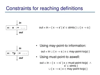
Reaching Definitions Contd. X=.. *p=.. Does definition of X reach here ? Yes Unambiguous Definition: X = ….; Ambiguous Definition: *p = ….; p may point to X For computing reaching definitions, typically we only consider kills by unambiguous definitions.
Computing Reaching Definitions d2: X=… d3: X=… IN[B] GEN[B] ={d1} d1: X=… KILL[B]={d2,d3} OUT[B] At each program point p, we compute the set of definitions that reach point p. Reaching definitions are computed by solving a system of equations (data flow equations).
Data Flow Equations IN[B]: Definitions that reach B’s entry. OUT[B]: Definitions that reach B’s exit. GEN[B]: Definitions within B that reach the end of B. KILL[B]: Definitions that never reach the end of B due to redefinitions of variables in B.
Reaching Definitions Contd. • Forward problem – information flows forward in the direction of edges. • May problem – there is a path along which definition reaches a point but it does not always reach the point. Therefore in a May problem the meet operator is the Union operator.
Applications of Reaching Definitions Constant Propagation/folding Copy Propagation
2. Available Expressions An expression is generated at a point if it is computed at that point. An expression is killed by redefinitions of operands of the expression. An expression A+B is available at a point if every path from the start node to the point evaluates A+B and after the last evaluation of A+B on each path there is no redefinition of either A or B (i.e., A+B is not killed).
Available Expressions Available expressions problem computes: at each program point the set of expressions available at that point.
Data Flow Equations IN[B]: Expressions available at B’s entry. OUT[B]: Expressions available at B’s exit. GEN[B]: Expressions computed within B that are available at the end of B. KILL[B]: Expressions whose operands are redefined in B.
Available Expressions Contd. • Forward problem – information flows forward in the direction of edges. • Must problem – expression is definitely available at a point along all paths. Therefore in a Must problem the meet operator is the Intersection operator. • Application: A
3. Live Variable Analysis Live Variable Analysis Computes: At each program point p identify the set of variables that are live at p. A path is X-clear if it contains no definition of X. A variable X is live at point p if there exists a X-clear path from p to a use of X; otherwise X is dead at p.
Data Flow Equations IN[B]: Variables live at B’s entry. OUT[B]: Variables live at B’s exit. GEN[B]: Variables that are used in B prior to their definition in B. KILL[B]: Variables definitely assigned value in B before any use of that variable in B.
Live Variables Contd. • Backward problem – information flows backward in reverse of the direction of edges. • May problem – there exists a path along which a use is encountered. Therefore in a May problem the meet operator is the Union operator.
Applications of Live Variables Register Allocation Dead Code Elimination
Conservative Analysis Optimizations that we apply must be Safe => the data flow facts we compute should definitely be true (not simply possibly true). Two main reasons that cause results of analysis to be conservative: 1. Control Flow 2. Pointers & Aliasing
Conservative Analysis X+Y is always available if we exclude infeasible paths. 1. Control Flow – we assume that all paths are executable; however, some may be infeasible.
Conservative Analysis 2. Pointers & Aliasing – we may not know what a pointer points to. 1. X = 5 2. *p = … // p may or may not point to X 3. … = X Constant propagation: assume p does point to X (i.e., in statement 3, X cannot be replaced by 5). Dead Code Elimination: assume p does not point to X (i.e., statement 1 cannot be deleted).
Representation of Data Flow Sets • Bit vectors – used to represent sets because we are computing binary information. • Does a definition reach a point ? T or F • Is an expression available/very busy ? T or F • Is a variable live ? T or F • For each expression, variable, definition we have one bit – intersection and union operations can be implemented using bitwise and & or operations.