Download
1 / 59
590 likes | 743 Views
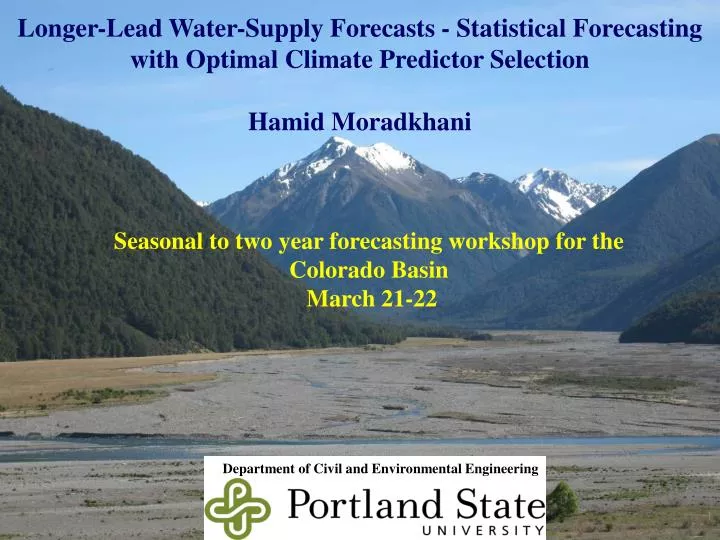
Longer-Lead Water-Supply Forecasts - Statistical Forecasting with Optimal Climate Predictor Selection Hamid Moradkhani. Seasonal to two year forecasting workshop for the Colorado Basin March 21-22. Department of Civil and Environmental Engineering. Background and Motivation.

E N D
Longer-Lead Water-Supply Forecasts - Statistical Forecasting with Optimal Climate Predictor Selection Hamid Moradkhani Seasonal to two year forecasting workshop for the Colorado Basin March 21-22 Department of Civil and Environmental Engineering
Background and Motivation • Interest in water supply forecasting has grown prominently in the western US • due to population growth and increasing demands for water • In the Western US, the NWRFC and the NRCS jointly issue seasonal water • supply outlook (WSO) forecasts of naturalized or unimpaired flow • Successful management of the West’s water supply is necessary to provide an • uninterrupted and dependable water supply to meet all the needs • One important aspect of successfully managing the West’s supply of water • is accurate and reliable forecasts of seasonal streamflow volumes • Longer-lead forecasts are useful to water managers and decision makers • but difficult to make due to the uncertainty in future winter and spring climate • conditions and the lack of snowpack information
Model selection: Statistical regression-based models A regression model consists of Dependent variable Predictor variable(s) A regression model established a linear relationship between the predictor variable(s) and the dependent variable (predictand) Developing a Forecast Model
The dependent variable is the total volumetric flow over a particular period at a specific point in a basin. Developing a Forecast Model Total Volumetric Flow = Sum(Apr to Sept Volumes) Total volume is what we want to predict
The Yakima River is located in central Washington in the Yakima River Basin and is approximately 215 miles in length. The Yakima Basin drains approximately 6,150 square miles of area. The basin is bordered on the west by the Cascade Mountains, on the north by the Wenatchee Mountains, on the east by the Columbia, and on the south by the Simcoe Mountains. The climate in most of the basin is dry, with a mean annual precipitation over the entire basin of 27 inches. Most of the precipitation in the basin falls during the winter months as snow in the mountains. Yakima River Basin
The Sprague River is located in southwestern Oregon in the Upper Klamath River Basin and is approximately 75 miles in length. The Sprague River drains an area east of the Cascade Mountains that is approximately 1,600 square miles in area. The climate in most of the basin is much drier than that of western Oregon, and has more extreme temperatures, especially in the winter months. Snowfall accounts for 30 percent of the annual precipitation in the valleys and as much as 50 percent in the mountains. Sprague River Basin
The Rogue River is located in southwestern Oregon in the Rogue River Basin and is approximately 220 miles in length. The Rogue River drains an area between the Cascade Mountains and the Pacific Ocean that is approximately 5,160 square miles. The climate of southwestern Oregon is cool and wet in the winter and among the hottest and driest in the western Cascades in the summer. Mean annual precipitation in the headwaters of the basin range from 20 to 30 inches, and 80 to 100 inches near the Oregon coast. Rogue River Basin
Sprague River Basin Basin location: Southwestern Oregon Basin size: 1,600 square miles Rogue River Basin Basin location: Southwestern Oregon Basin size: 5,160 square miles Study Basins MAP (in) MAP (in) Streamflow (1000-AF) Streamflow (1000-AF) Month Month MAP (in) Yakima River Basin Basin location: Central Washington Basin size: 6,150 square miles Streamflow (1000-AF) Month
Our objective is to establish a linear relationship between several predictor variables (x), and a predictand (y) Given a set of data that consists of n observations and j predictor variables the problem becomes finding the regression function Each of the j predictor variables has its own regression parameters, bj, and regression constant, b0. The best possible estimates of the regression parameters are the ones which minimize the sum of the squared errors Developing a Forecast Model
Explore the relationship between streamflow and: Snow water equivalent Precipitation for past months Streamflow for past months Streamflow in the West is the result of the Accumulation of seasonal snowpack over the winter months Melting of this snowpack over the spring and summer Identifying Potential Predictors
Fall and winter precipitation can also provide information about spring runoff This gives us information about the soil moisture state in the basin Identifying Potential Predictors Total Fall and Winter Precipitation = Sum(Oct to Forecast Issue Date)
Past months streamflow also provides useful information about future streamflow volumes. Combining these three predictors would results in the following: Identifying Potential Predictors Forecast Issue Date SWE Antecedent Precipitation Forecast Window Antecedent Streamflow • Jan Feb Mar Apr May Jun Jul Aug Sep Oct Nov Dec Jan Feb Mar Apr - Sep
Recent research has shown that forecast accuracy can be improved by including large-scale climate information into forecasts models. Some useful climate teleconnection indices commonly used for streamflow forecasting in the western US: Southern Oscillation Index (SOI) Pacific Decadal Oscillation (PDO) Multivariate El Nino Southern Oscillation Index (MEI) Pacific North American Index (PNA) Trans-Nino Index (TNI) Identifying Potential Predictors
So how do we incorporate large-scale climate information into seasonal forecasts… Goal: Establish a relationship between climate information and spring runoff. Analysis: Investigate how climate information from the previous year relates to spring runoff of the forecast year. Identifying Potential Predictors
Correlation analysis can be performed by taking monthly or 3-month aggregations of climate data and correlating with spring runoff. Identifying Potential Predictors
Combining SWE, climate information from past months, precipitation from past months, and streamflow from past months Identifying Potential Predictors Forecast Issue Date SWE 3-Month Climate Data Antecedent Precipitation Forecast Window Antecedent Streamflow • Jan Feb Mar Apr May Jun Jul Aug Sep Oct Nov Dec Jan Feb Mar Apr - Sep
We have a set of potential predictors that capture some of the physical driving processes of streamflow, now how do we use them in a regression model? Looking at the data we would find that our predictors are intercorrelated. Identifying Potential Predictors
If the predictor variables have minimal correlation among themselves, then application of the OLS regression methodology works as intended. If, on the other hand, the predictor variables are mutually correlated, then the predictor variables contain redundant information, and this condition leads to parameter estimates that are biased. Several remediation techniques are available for dealing with datasets that would otherwise give bias parameter estimations. Principal component regression Partial least squares regression Z-score regression Independent component regression Intercorrelated Predictor Variables
Principal component regression (PCR) combines principal component analysis (PCA) with multiple linear regression. PCA is a technique that creates new variables from the original predictor variables that can be scored and ordered. Principal components: are composites of many of the original predictor variables they represent a smaller number of variables that maintain the important patterns in the data. Principal components are generated from linear combinations of the predictor variables. Principal Component Regression
Principal components are ordered The first principal component accounts for as much of the variability in the data set as possible Each succeeding component accounts for as much of the remaining variability as possible. Most importantly, the principal components created from PCA are uncorrelated, which allows them to be used in multiple linear regression. Principal Component Regression
PCR Steps: Start by standardizing the predictor dataset – subtract the sample mean and divide by the sample standard deviation. Compute the sample variance-covariance matrix of the standardized dataset. Calculate the eigenvectors and eigenvalues of the variance-covariance matrix. Calculate the principal component time series by multiplying each predictor variable times the corresponding eigenvector. Use the principal components obtained from step 4 in linear regression model. Principal Component Regression
PCA produces the same number of principal components as there are predictor variables. Some measure must be used to select the number of principal components to retain in the regression model. We investigated two methods: The regression parameters are tested using a standard t-test and a user specified critical t-value The Prediction REsidualSum of Squares (PRESS) statistic is calculated using a leave one out cross-validation procedure Principal Component Regression
Principal components are added into the regression model one-by-one The addition of each principal component is checked for statistical significance using the standard t-test. The principal components are retained in the regression model as long as the regression parameters are statistically significant (t-value > 1.6). Principal Component Regression
The PRESS statistic is calculated for each of the extracted factors j using: PRESS(j) = ∑(qobs – qsim(j))2 Where qobs observed streamflow value qsim (j) predicted streamflow value for the extracted factor j The PRESS statistic with the minimum value is then used to determine the number of extracted components to keep in the final model. Principal Component Regression
Partial least squares regression (PLSR) is based on the principal components of both the predictor (X) and the dependent variable (Y) PLSR is different than PCR in that PLSR searches for a set of components that explains the maximum covariance between X and Y, where PCR concentrates on the variance of X only PLSR decomposes X and Y into a score matrix (Sx, Sy) times a loading matrix (Lx, Ly) and a residual matrix (Ex, Ey): X = Sx * Lx + Ex Y = Sy * Ly + Ey This is referred to as the outer relations Partial Least Squares Regression
PLSR seeks to minimize Ey while maintaining the correlation between X and Y by an inner relations: X = Sx * Lx + Ex (1) Y = Sy * Ly + Ey(2) Sy = D * Sx + Ei (3) Where, D = diagonal correlation matrix between X and Y Ei = error term Inserting equation (3) into equation (2) gives a predictive model for Y Y = D * Sx * Ly + Eyy where Eyy is to be minimized Partial Least Squares Regression Outer relations Inner relations
PLSR also produces the same number of components as there are predictor variables. In this study the PRESS statistic is used for determining the optimal number of components to retain PRESS(j) = ∑(qobs – qsim(j))2 Where qobs observed streamflow value qsim (j) predicted streamflow value for the extracted factor j Partial Least Squares Regression
This research investigated the use of Independent Component Analysis (ICA) for the decomposition of large-scale climate data in order to see if statistically significant climate predictors could be extracted. The idea is that the oceanic and atmospheric systems receive contributions from many sources and that the observations represent a linear mixture of independent signals. Before ICA was implemented a quick correlation analysis was performed using the NCEP Reanalysis data provided by the Physical Sciences Division NOAA/OAR/ESRL (http://www.cdc.noaa.gov/). Development of Climate Predictors using ICA
Climate Signal Correlation With Apr-Sept Streamflow Volume Yakima River Basin Rogue River Basin Sea Level Pressure Surface Air Temperature Surface Pressure Surface Air Temperature Geopotential Height Relative Humidity Geopotential Height Precipitable Water
ICA is a method that separates mutually independent signals from observation data The ICA model: X = A * S X = observed data A = some unknown mixing matrix S = independent components Assumptions: Observed signals are linear mixtures of unobserved independent signals Independent signals are non-Gaussian and mutually independent Independent Component Analysis
Independent Component Analysis What is ICA? “Independent component analysis (ICA) is a method for finding underlying factors or components from multivariate (multi-dimensional) statistical data. What distinguishes ICA from other methods is that it looks for components that are both Statistically Independentand NonGaussian.” The simple “Cocktail Party” Problem Mixing matrix A x1 s1 Observations Sources x2 s2 x1 = a11s1 + a12s2 x2 = a21s1 + a22s2 x = As n sources, m observations
Independent versus Uncorrelated Two variables of y1 and y2 are independent if and only if: P(y1,y2) = P1(y1)P2(y2) • Uncorrelatedness is a weaker form of independence. • When two variables are independent they are also uncorrelated however the inverse is not true.
The independent components must be non-Gaussian for ICA to be possible.Maximizing the non-Gaussianity of WTxresults in the independent components.
Measures of Non-Gaussianity • We need to have a quantitative measure of non-Gaussianityfor ICA Estimation. • Kurtosis : gauss = 0 (sensitive to outliers) • Entropy : Gauss = largest • Neg-entropy : Gauss = 0 (difficult to estimate) Approximations where v is a standard Gaussian random variable and :
ICA vs PCA • Principle Component Analysis (PCA) translates a set of possibly correlated variables into a set of values of uncorrelated variables which is called principal components. • Independent Component Analysis (ICA) goes beyond and finds independent variables. Therefore some preprocessing steps would make the problem of ICA estimation simpler: • Centering • Whitening
ICA Preprocessing • Centering: is achieved by subtracting the mean vector (m) from the mixed signal “x”. • After estimating the mixing matrix with centered data, one can add the mean vector of s (obtained from A-1) back to the centered estimates of s. • Whitening: to linearly transform the observed vector “x” so that its components are uncorrelated and their variances equal unity.
Independent Component Analysis Original Signals [So] Mixed Signal [X] Mixing Matrix [A]
Independent Component Analysis Estimated Signals [S] Mixed Signal [X] ICA
Independent Component Analysis Estimated Signals [S] Original Signals [So]
Seasonal Climate Signal Correlation with Rogue Apr-Sept Streamflow Volume NCEP/NCAR Reanalysis
Seasonal Climate Signal Correlation with Sprague Apr-Sept Streamflow Volume NCEP/NCAR Reanalysis
ICA climate predictor identification steps: Select one of the large-scale climate data sets to analyze. The climate data should consist of monthly values and will have dimensions n x m where n is the number of historical observations and m is the number of months. The number of historical observations, n, used in this study was 30 (1979-2008). Development of Climate Predictors using ICA
Perform the following steps itimes, where i = 1 to m: Use PCA to find i principal components for the selected climate data set. Whiten the data using the eigenvectors and eigenvalues from PCA above. Use ICA algorithm to estimate i independent components. In this study it is assumed that the number of signals is equal to the number of principal components. Retain each of the estimated iindependent components. The number of components retained, r, is given by r = m(m+1)/2. Calculate the Pearson’s correlation coefficient between each r independent climate signal and spring runoff. Retain the climate signal that has the highest correlation coefficient. Development of Climate Predictors using ICA
Repeat steps 2 through 3 k times, where k = 50 for this study. Repeating steps 2 through 3 is necessary because the ICA program implements a stochastic algorithm and the ICA decomposition is only unique up to sign, scaling and permutation. This bootstrapping technique is a way of ordering and selecting only those signals that are linearly correlated with spring runoff. The result of step 5 will be a matrix of dimensions n x k. Perform PCA on the matrix n x k from step 4 above, keeping only the first principal component. Whiten the data using the eigenvectors and eigenvalues from step 5. Perform ICA using the whitened data from step 6 to estimate one independent component. The result from this step is a n x 1 column vector which becomes the climate predictor variable in the multiple linear regression model. Development of Climate Predictors using ICA
ICA climate predictor selection for the Yakima River Basin New predictors have strong correlation with spring runoff ICA procedure found 9 new predictors to include in regression model
ICA climate predictor selection for the Rogue River Basin • New predictors have strong correlation with spring runoff • ICA procedure found 9 new predictors to include in regression model
ICA climate predictor selection for the Sprague River Basin • New predictors have strong correlation with spring runoff • ICA procedure found 7 new predictors to include in regression model


![Statistical Forecasting [Part 1]](https://cdn3.slideserve.com/6737421/statistical-forecasting-part-1-dt.jpg)