Remote sensing using noise

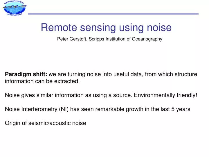
1. Remote sensing using noise Peter Gerstoft, Scripps Institution of Oceanography Paradigm shift: we are turning noise into useful data, from which structure information can be extracted. Noise gives similar information as using a source. Environmentally friendly! Noise Interferometry (NI) has seen remarkable growth in the last 5 years Origin of seismic/acoustic noise

2. Super Typhoon Ioke (in 2006)

3. Tracking Tropical Cyclones Zhang, Gerstoft, and Bromirski (under review) • Evidencing nonlinear wave-wave interactions in the deep ocean • (Longuet-Higgins, 1950) • Tracking wave-wave interactions rather than a storm itself

4. Track of storm from microseisms (0.2 Hz)

5. Mechanism involves ocean acoustics! Ocean waves Deep ocean bottom Classic seismic P-wave propagation

6. Free space noise correlation τ=0 * * τ=L/c 1 2 ENDFIRE DIRECTION Sources yielding constant time-delay τ lay on same hyperbola 2→1 1→ 2 C12(τ) τ 0 -L/c +L/c

7. Wd=80 m 230 m long array Ambient noise EGFs (20-100 Hz) EGF envelopes (dB) with modeled travel times (dotted) between hydrophones Distance (m) Time (s) Amplitude (dB) Brooks and Gerstoft (JASA 2009a 2009b); Fried at al (JASAEL 2008)

8. Green’s functions estimate Wd=70 m 230 m long array • Vertical lowered source • Towed source • Ship noise • Ambient noise

9. origin 1 20 3 21 2 Noise array localization • Methodology adapted from Sabra [2005] • HLA elements parameterized by distance and azimuth: model vector : • Travel times from peak of empirical Green’s function: observed data vector: • A priori arrayisstraight • Objective function minimize difference between observed traveltimes and computed traveltimes from model vector, whilst ensuring “smooth” fit • Objective functionminimized usingMATLAB’snonlinear least-squares function • Six largest travel-time difference rejected for each computation • Lower and upper limits set to half and twice a priori distances • Variation of the smoothness ‘weighting’ seen to have negligible effect

10. A priorivsa posteriori geometry A posteriori geometry A priori geometry

11. B1 B2 Passive fathometer Using ambient noise on a drifting array we can map the bottom properties Siderius et al., JASA 2006, Gerstoft et al., JASA 2008, Harrison, JASA 2008 Harrison, JASA 2009, Traer et al., JASA 2009, Siderius et al., JASA 2010

12. Fathometer comparison to seismic South of Sicily (NURC: 32 phones spaced at 0.5 m) Dabob Bay, Wa (16 phones spaced at 0.5 m) Gerstoft et al., JASA 2008,

13. Active source (Uniboom) Background Passive fathometer MVDR Passive fathometer Siderius. JASA, 2010

14. Retrieving temporal velocity variations dt A temporal change in velocity along the path between two stations is revealed as an increase in dt with propagation distance, when comparing the cross-correlations from two different time periods.

15. Velocity change across a fault Measured velocity change associated with damage from earthquakes and volcanic precursors. Brenguier et al, Science 2008

16. Conclusion • Noise provides useful signal • We can obtain a partial Greens function Applications: • Locating noise sources • Used for obtaining Earth structure (many applications) • Fathometer • Structural health monitoring • Human body monitoring

17. Up Down Downward beam (MAPEX2000bis) 32 element NURC array Angle Above design frequency, downgoing noise appears as upgoing Frequency (kHz) SW06: d=4m => No fathometry! We need dense arrays to get sufficient resolution. New Siderius arrays (d~0.5m) makes fathometry feasible.

18. Ernesto Seismic Beamforming: a seismic array in California detected low frequency signals on Sep 2 from a direction consistent with the SW06 site. => Stay ashore Ernesto provided ideal conditions for noise cross-correlation

19. Model for amplitudes • Coherent averaging • Averaging time • Is the array moving up and down? Future fathometer work Experimental data shows array is subject to wave driven motion, preventing coherent averaging

20. P Waves Imaging Earth Structure Teleseismic body-wave tomography (regional) ? Humphreys & Clayton (JGR, 1990) Polet (G3, 2007) Storms (seismic sources in open ocean) can fill azimuth gaps Storms

21. History of seismic/acoustic interferometry • 1968 Claerbout • 1980’s experiment at Stanford • 1990’s helioseismology • 2001 Weaver and Lobkis • 2004 first papers in seismology, & ocean acoustics (Roux and Kuperman) • 2008 book “Seismic interferometry: History and present status” • 2009 book “Seismic interferometry” • 2009 ~100 papers/year; 3 in Science or Nature /year Progress due to better computer resources, instrumentation and theory. Still lots of low hanging fruits!

23. Ocean noise interferometry publications www.mpl.ucsd.edu/people/pgerstoft • Traer, Gerstoft and Hodgkiss (2010), Ocean bottom profiling with ambient noise: a model for the passive fathometer, submitted JASA. • Siderius, Song, Gerstoft, Hodgkiss, Hursky, Harrison (2010), Adaptive passive fathometer processing, JASA. • Brooks, Gerstoft (2009), Green’s function approximation from cross-correlation of active sources in the ocean, JASA. • Brooks, Gerstoft (2009), Green's function approximation from cross-correlations of 20–100 Hz noise during a tropical storm, JASA. • Traer, Gerstoft, Song. Hodgkiss (2009), On the sign of the adaptive passive fathometer impulse response, JASA. • Gerstoft, Hodgkiss, Siderius, Huang, Harrison (2008), Passive fathometer processing, JASA. • Brooks, Gerstoft, Knobles (2008), Multichannel array diagnosis using noise cross-correlation, JASA EL. • Traer, Gerstoft, Bromirski, Hodgkiss, Brooks (2008), Shallow-water seismo-acoustic noise generation by Tropical Storms Ernesto and Florence, JASA EL. • Brooks and Gerstoft (2007), Ocean acoustic interferometry, JASA, • Tomorrow: Bill Hodgkiss nearfield geoacoustic inversion Caglar Yardim PF and objective functions