Download
1 / 52
530 likes | 658 Views
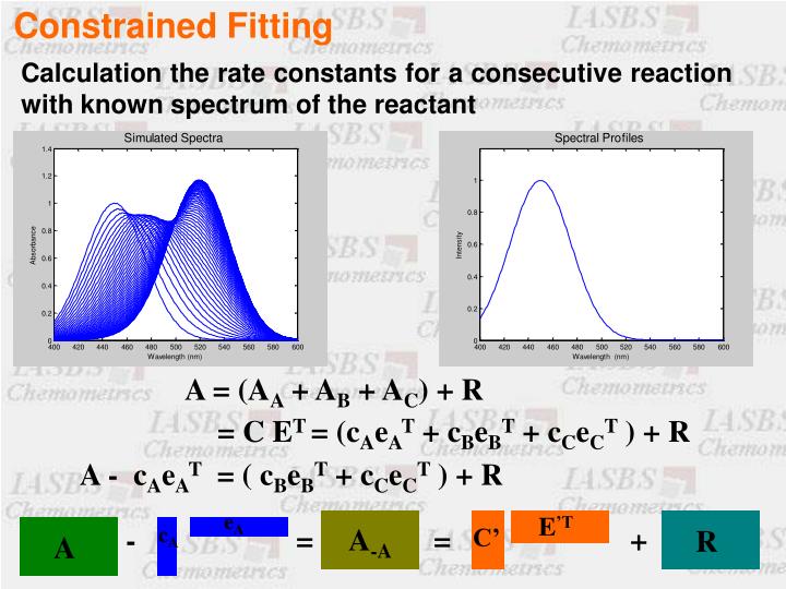
Constrained Fitting. e A. E ’T. c A. A -A. C’. A. R. Calculation the rate constants for a consecutive reaction with known spectrum of the reactant. A = (A A + A B + A C ) + R. = C E T = (c A e A T + c B e B T + c C e C T ) + R. A - c A e A T = ( c B e B T + c C e C T ) + R.

E N D
Constrained Fitting eA E’T cA A-A C’ A R Calculation the rate constants for a consecutive reaction with known spectrum of the reactant A = (AA + AB + AC) + R = C ET = (cAeAT + cBeBT + cCeCT ) + R A - cAeAT = ( cBeBT + cCeCT ) + R - = = +
r_cons2.m Calculation the residual based on known spectrum of reactant
? Compare the errors of parameters with and without known spectrum of reactant.
? How selectivity constraint (zero region) can be applied in calculation the residual vector?
Chemical Kinetics Modeling by Numerical Solving of Ordinary Differential Equations
Calculation of kinetic concentration profiles k1 A B k1 k2 A B C k2 d[A] = -k1 [A] dt d[A] d[B] = -k1 [A] + k2 [B] dt = k1 [A] - k2 [B] dt d[B] = k1 [A] - k2 [B] d[C] dt = k2 [B] dt The central step in the fitting of a kinetic model to multivariate measured data is being able to calculate the concentration profiles of the species involved in a chemical reaction. A = C E + R According to kinetic theory, the concentration prfiles of the species in a reaction mechanisms are defined by a system of ordinary differential equations (ODEs)
k1 k2 A B C k4 k3 D d[A] = -k1 [A] dt d[B] = k1 [A] - k2 [B] –k3 [B] + k4 [D] dt d[C] = k2 [B] dt d[D] = k3 [B] – k4[D] dt Complex Reactions
d[A] = -k1 [A] – k3 [A] dt k3 A D + E d[B] = k1 [A] – k2 [B] – k4[B] k1 k6 dt k4 B D + F d[C] = k2 [B] – k5 [C] dt k2 k7 k5 d[D] C D + G = k3 [A] + k4 [B] + k5[C] dt d[E] = k3 [A] – k6 [E] dt d[F] = k6 [E] + k4 [B] – k7[F] dt d[G] = k7 [F] + k5 [C] dt
Numerical Integration of ODEs system There is a limited number of reaction mechanisms for which there are explicit formulae to calculate the concentrations of the reacting species as a function of time. To overcome this, numerical integration is used. Numerical integration allows an approximation to the explicit solution to be calculated for any system of ODEs, within limits of numerical accuracy and computation time. An example d(A] k1 = -2 k1 [A] 2 2 A B dt k2 d(B] B C = k1 [A] 2 - k2[B] dt [A]0 =1 d(C] = k2[B] [B]0 =[C]0=0 dt
The Euler Method f (x + Dx) = f (x) + ( ) (Dx) + ( ) (Dx)2 df (x) dnf (x) d2f (x) df (x) 1 1 + … + ( ) (Dx)n d x d2x dn x d x 2! n! f (x + Dx) = f (x) + ( ) (Dx) The Euler method is the simplest method for the numerical integration of a system of differential equations. It can be seen as an adaptation of the truncated Taylor series expansion. The Taylor series expansion C at t0 is C0 C(t0 +Dt)= C(t0) + (dC(t0)/dt)Dt What is C at t=t0 +Dt ?
The Euler Method d(A] [A]0 =1 If k1=0.2 k2=0.4 = -2 k1 [A] 2 dt [B]0 =[C]0=0 for Dt = 0.2 [A] 1 = [A] 0 + (d[A]0 / dt)Dt (d[A]0 / dt)= - 2(0.2)(1)2 = - 0.4 [A] 1 = 1 – (0.4) (0.2) = 0.92 [A] 2 = [A] 1 + (d[A]1 / dt)Dt (d[A]1 / dt)= - 2(0.2)(0.92)2 = -0.3386 [A] 2 = 0.92 – (0.3386) (0.2) = 0.8523
Effect of time increment on calculated concentration profiles by Euler method dt1=0.1 dt2=0.2 dt3=0.4 dt4=0.6 dt5=0.8 dt6=1
k1 A B k2 Modify the euler.m file for calculating the concentration profiles for the following mechanism: ?
Fourth Order Runge-Kutta Method The main disadvantage of the Euler method is that the calculated approximation for the concentrations are systematically wrong for each step. For a good accuracy, step sizes have to be very small. Fourth order Runge-Kutta method is a modification of Euler method. It is called fourth order because the first derivative is calculated at four points along the increment of integration, allowing much larger increments and thus dramatically reduced computation times compared to the simple Euler method.
Fourth Order Runge-Kutta Method d(A] k1 = -2 k1 [A] 2 2 A B dt k2 d(B] B C = k1 [A] 2 - k2[B] dt [A]0 =1 d(C] = k2[B] [B]0 =[C]0=0 dt If k1=0.4 k2=0.2 Step 1 Calculating the derivatives of the concentration at t0 (d[A]0 / dt)= - 2(0.4)(1)2 = - 0.8 (d[B]0 / dt)= (0.4)(1)2 – (0.2)(0) = 0.4 (d[C]0 / dt)= (0.2)(0) = 0
Fourth Order Runge-Kutta Method Step 2 Calculating approximate concentration at the intermediate time point, Dt/2 based on concentration and derivative at t0 [A] 1 = [A] 0 + (d[A]0 / dt)Dt/2 [A] 1 = 1 – (0.8) (0.1) = 0.92 [B] 1 = [B] 0 + (d[B]0 / dt)Dt/2 [B] 1 = 0 + (0.4) (0.1) = 0.04 [C] 1 = [C] 0 + (d[C]0 / dt)Dt/2 [C] 1 = 0 + (0) (0.1) = 0
Fourth Order Runge-Kutta Method Step 3 Calculating the derivatives at the intermediate time point. (d[A]1 / dt)= - 2(0.4)(0.92)2 = - 0.6771 (d[B]1 / dt)= (0.4)(0.92)2 – (0.2)(0.04) = 0.3306 (d[C]1 / dt)= (0.2)(0.04) = 0.008
Fourth Order Runge-Kutta Method Step 4 Calculating another set of concentrations at the intermediate time point, now based on concentration at time 0 and derivatives at the intermediate time point. [A] 2 = [A] 0 + (d[A]1 / dt)Dt/2 [A] 2 = 1 – (0.6771) (0.1) = 0.9323 [B]2 = [B] 0 + (d[B]1 / dt)Dt/2 [B] 2 = 0 + (0.3306) (0.1) = 0.03306 [C] 2 = [C] 0 + (d[C]1 / dt)Dt/2 [C] 2 = 0 + (0.008) (0.1) = 0.0008
Fourth Order Runge-Kutta Method Step 5 Calculating a new set of derivatives at the intermediate time point, based on the concentration just calculated (d[A]2 / dt)= - 2(0.4)(0.9323)2 = -0.6953 (d[B]2 / dt)= (0.4)(0.9323)2 – (0.2)(0.03306) = 0.3411 (d[C]2 / dt)= (0.2)(0.03306) = 0.00661
Fourth Order Runge-Kutta Method Step 6 Calculating the concentration at the new time point 1, after the complete time interval, based on the concentration at to and these new derivatives at the intermediate time point: [A] 3 = [A] 0 + (d[A]2 / dt)Dt [A] 3 = 1 – (0.6953) (0.2) = 0.8609 [B]3 = [B] 0 + (d[B]2 / dt)Dt [B] 3 = 0 + (0.3411) (0.2) = 0.0682 [C] 3 = [C] 0 + (d[C]2 / dt)Dt [C] 3 = 0 + (0.00661) (0.2) = 0.0013
Fourth Order Runge-Kutta Method Step 7 Computation of derivatives at time point 1: (d[A]3 / dt)= - 2(0.4)(0.8609)2 = -0.5929 (d[B]3 / dt)= (0.4)(0.8609)2 – (0.2)(0.0682) = 0.2828 (d[C]3 / dt)= (0.2)(0.0682) = 0.0136
d[A]0/dt) + 2 (d[A]1/dt) + 2(d[A]2/dt) +(d[A]3/dt) d[A]new/dt) = 6 Fourth Order Runge-Kutta Method Step 8 Computation the new concentration after the ful time interval based on weighted average of derivatives [A] new = [A] 0 + (d[A]new / dt)Dt [A] 3 = 1 – (0.6896) (0.2) = 0.8621 [B]new = [B] 0 + (d[B]new / dt)Dt [B] 3 = 0 + (0.3377) (0.2) = 0.0675 [C] new = [C] 0 + (d[C]new / dt)Dt [C] 3 = 0 + (0.0071) (0.2) = 0.0014
ODE1.m Fourth Order Runge-Kutta Method and MATLAB
Dt=0.1 RK Dt=0.5 RK Dt=0.5 E Comparison of results from Euler and Runge-Kutta methods with same time increment
k1 A B k2 Use Runge-Kutta method for calculating the concentration ptofiles for the following mechanism: ?
k1 A B k2 d[A] = -k1 [A] + k2 [B] dt d[B] = k1 [A] - k2 [B] dt Generalized model for different kinetic mechanisms n1 = k1 [A] = k1 [A]1 [B]0 n2 = k2 [B] = k2 [A]0 [B]1 d[A] = (-1) n1 + (1) n2 dt d[B] = (1) n1 + (-1) n2 dt
k1 k2 A B C d[A] = -k1 [A] dt d[B] = k1 [A] - k2 [B] dt d[C] = k2 [B] dt Generalized model for different kinetic mechanisms n1 = k1 [A] = k1 [A]1 [B]0 [C]0 n2 = k2 [B] = k2 [A]0 [B]1 [C]0 d[A] = (-1) n1 + (0) n2 dt d[B] = (1) n1 + (-1) n2 dt d[C] = (0) n1 + (1) n2 dt
Generalized model for different kinetic mechanisms k1 2 A B k2 B C d(A] n1 = k1 [A]2 = k1 [A]2 [B]0 [C]0 = -2 k1 [A] 2 dt n2 = k2 [B] = k2 [A]0 [B]1 [C]0 d(B] = k1 [A] 2 - k2[B] dt d[A] = (-2) n1 + (0) n2 d(C] dt = k2[B] dt d[B] = (1) n1 + (-1) n2 dt d[C] = (0) n1 + (1) n2 dt
Generalized model for different kinetic mechanisms n1 = k1 [A] = k1 [A]1 [B]0 n1 = k1 [A] = k1 [A]1 [B]0 [C]0 n2 = k2 [B] = k2 [A]0 [B]1 n2 = k2 [B] = k2 [A]0 [B]1 [C]0 d[A] d[A] = (-1) n1 + (1) n2 = (-1) n1 + (0) n2 dt dt d[B] d[B] = (1) n1 + (-1) n2 dt = (1) n1 + (-1) n2 dt n1 = k1 [A]2 = k1 [A]2 [B]0 [C]0 d[C] = (0) n1 + (1) n2 n2 = k2 [B] = k2 [A]0 [B]1 [C]0 dt d[A] = (-2) n1 + (0) n2 dt d[B] = (1) n1 + (-1) n2 dt d[C] = (0) n1 + (1) n2 dt
Generalized model for different kinetic mechanisms n1 = k1 [A]2 = k1 [A]2 [B]0 [C]0 n2 = k2 [B] = k2 [A]0 [B]1 [C]0 d[A] = (-2) n1 + (0) n2 dt d[B] = (1) n1 + (-1) n2 dt d[C] = (0) n1 + (1) n2 dt k1 Reactant stoichiometries matrix, Xr 2 A B A B C k2 B C k1 2 0 0 k2 0 1 0 Product stoichiometries matrix, Xp A B C k1 0 1 0 k2 0 0 1 Stoichiometric coefficient matrix, X = Xp - Xr A B C k1 -2 1 0 k2 0 -1 1
Generalized model for different kinetic mechanisms Once Xr and X have been determined, the differential equations can be constructed in a completely generalized way. nj is the rate law of the j-th elementary step in the mechanism. ns Xr j, i P ci nj= kj where j=1 to np i=1 np S d ci Xj, i nj = where i=1 to ns dt j=1
kinfun.m A generalised function for creating the ODEs system
GKIN.m generalised modeling the reaction kinetics with known mechanism
Using GKIN.m file for modeling k1 2 A B k2 B C Reactant stoichiometries matrix, Xr A B C k1 2 0 0 k2 0 1 0 Product stoichiometries matrix, Xp A B C k1 0 1 0 k2 0 0 1
Reactant stoichiometries matrix, Xr A B C k1 2 0 0 k2 0 1 0
Product stoichiometries matrix, Xr A B C k1 0 1 0 k2 0 0 1