Download
1 / 43
430 likes | 546 Views
Confinement of spin diffusion to single molecular layers in layered organic conductor crystals. I.F. Schegolev Memorial Conference “Low-Dimensional Metallic and Superconducting Systems” October 11–16, 2009, Chernogolovka, Russia. András Jánossy 1 Ágnes Antal 1 Titusz Fehér 1

E N D
Confinement of spin diffusion to single molecular layers in layered organic conductor crystals I.F. Schegolev Memorial Conference “Low-Dimensional Metallic and Superconducting Systems” October 11–16, 2009, Chernogolovka, Russia András Jánossy1 Ágnes Antal1 Titusz Fehér1 Richard Gaál2 Bálint Náfrádi1,2 László Forró2 Crystal growth: Erzsébet Tátrainé Szekeres1, Ferenc Fülöp1 special thanks to Natasha Kushch 1Budapest University of Technology and Economics, Institute of Physics 2Ecole Polytechnique Federale de Lausanne
Quasi 2D molecular layered compounds: Independent currents in each layer? Uncoupled magnetic order in each layer? IAor MA A IBor MB B A B
- ET2-X, layered organic crystal X = Cu[N(CN)2]Cl, Br 2D polymer b 1 hole / ET2 dimer c A X B a ac=90° ac=0°
- ET2-X, layered organic crystal X = Cu[N(CN)2]Cl, Br 2D polymer b 1 hole / ET2 dimer c A tII t X B a t// 100 meV ac=45° t 0.1 meV
Phase diagram-(BEDT-TTF)2CuN(CN)2Cl, Br Mott transition 1 5 10
Goal: Determine: 1. interlayer magnetic interaction in antiferromagnet 2. interlayer electron hopping frequency, in metallic phase Method: high frequency ESR 1. Antiferromagnetic resonance, AFMR 2. Conduction electron spin resonance, CESR
High frequency ESR spectrometer high resolution same sensitivity 0-12 kbar pressure 420 GHz, Lausanne 222.4 GHz, Budapest 9.4 GHz BRUKERE500
Phase diagram-(BEDT-TTF)2CuN(CN)2Cl, Br ET-Cl ET-Br 2. Conduction electron spin resonance 1 5 10 1. Antiferromagnetic resonance
Antiferromagnetic resonance F = HZeeman + Hexchange + HDM + Hanisotropy F = - B(M1 + M2 ) + M1 M2 + D(M1 x M2) + ½Kb(M1y2 +M2y2)+½K(M1z2 + M2z2) D z y M1 M2 B 2 magnetizations 2 oscillation modes First AFMR work: Ohta et al, Synth. Met, 86, (1997), 2079-2080
Magnetic structure DA J = 600 T MA1 A MA2 lAB =? B DB MB2 D. F. Smith and C. P. Slichter, Phys. Rev. Let. 93, 167002, 2004 F = FA + FB+ lABMAMB MB1
Antiferromagnetic resonance calculation-(BEDT-TTF)2CuN(CN)2Cl B // b F = FA + FB+ lABMAMB ωb ωa 4 magnetizations : 4 modes: ωαA , ωbA ωαB , ωbA Frequency [GHz] 111.2 GHz Magnetic field [T] Antal et al., Phys. Rev. Lett. 102, 086404 (2009)
Antiferromagnetic resonance experiment-(BEDT-TTF)2CuN(CN)2Cl AFMR, 111.2 GHz, 4 K, H//b F = FA + FB+ lABMAMB 4 magnetizations : 4 modes: ωαA , ωbA ωαB , ωbA Antal et al., Phys. Rev. Lett. 102, 086404 (2009)
Antiferromagnetic resonance measured and calculated b B, magnetic field A ab a lAB B A and B modesdonotcross! intra-layerexchange: J = 600 T inter-layercoupling:AB =1x 10⁻³ T AB = AB exchange+ ABdipole (sameorder of magnitude) Antal et al., Phys. Rev. Lett. 102, 086404 (2009)
Conduction electron spin resonance in the metallic phase ET-Cl ET-Br Conduction electron spin resonance 1 5 10
2D spin diffusion A B interlayer hopping rate T1spin life time < 1/T1 2D spin diffusion
2D spin diffusion spin ≈ 250 nm vF//= 1 nm A t B = (2t2 //)/ ħ 2blocked by short // N. Kumar, A. M. Jayannavar, Phys. Rev. B 45, 5001 (1992) Expectation (300 K) : ħ / t≈10-11 s, //≈ 10-14 s T1≈ 10-9 s ≈ 2x10⁸ s < 1/T1 2D spin diffusion
Measurement of interlayer hopping ESR of 2 coupled spins A= gABB/h A B= gBBB/h B gA ≠ gB
Measurement of interlayer hopping ESR > I A – BI B A interlayer hopping frequency ≈ I A – BI B A < I A – BI B A
2 resolved ESR lines P=0, T=45-300 K A A B Ref. B < I A – BI < 3 x 10⁸ Hz Antal et al., Phys. Rev. Lett. 102, 086404 (2009)
ESR g- factor anisotropy 45 -250 K -(BEDT-TTF)2CuN(CN)2Cl b B, magnetic field a a B A Antal et al., Phys. Rev. Lett. 102, 086404 (2009)
Measurement of interlayer hopping ESR > I A – BI B A interlayer hopping frequency pressure ≈ I A – BI B A < I A – BI B A
Measurement of interlayer hopping Motional narrowing under pressure 210 GHz T=250 K, B in (a,b) plane -ET2-Cl Ref. Instr. > I A – BI ≈ I A – BI pressure < I A – BI
Measurement of interlayer hopping Motional narrowing under pressure 420 GHz T=250 K, A ESR spectral intensity B = I A – BI = 1.0 x10⁹ s-1
Measurement of interlayer hopping pressure dependence T=250 K = (2t2 //)/ħ2 blocked interlayer hopping // parallel d.c. conductivity
Summary (P, T) interlayer hopping frequency ET-Cl ET-Br 2x10⁸ s-1 5x10⁹ s-1 1 5 10
Measurement of interlayer hopping temperature dependence 111.2 GHz P=0 metal temperature Interlayer hopping frequency antiferromagnet
Measurement of interlayer hopping temperature dependence 111.2 GHz P=4 kbar metal temperature Interlayer hopping frequency superconductor
2D spin diffusion confinement ≈ 350 nm A vF//= 1 nm B = (2t2 //)/ ħ 2blocked by short // Measurement 250 K, P=0 : ≈ 2x10⁸ s-1 < 1/T1 2D spin diffusion Electrons are confined to single molecular layers in regions of 350 nm radius // = 10-14 - 10-13 s t= 0.1 meV - 0.03 meV
Anisotropy of resistivity t// 100 meV t 0.1 meV H. Ito et al J. Phys. Soc. Japan 65 2987 (1996) • / // nearly independent of T • 100 cm • / // 102 - 103
Anisotropy of resistivity -(BEDT-TTF)2CuN(CN)2Br -(BEDT-TTF)2CuN(CN)2Cl Buravov et al. J. Phys. I 2 1257(1992) H. Ito et al J. Phys. Soc. Japan 65 2987 (1996) = (2t2 //)/ ħ 2 blocking of interlayer tunnelling 1 / 1 / //, // 1 / // / // ( t// / t )2 (a/d)2 independent of T
Perpendicular dc resistivity: = 1/( e2 g(EF) d) g(EF) = two dimensinal density of states d: interlayer distance -(BEDT-TTF)2CuN(CN)2Cl at 250 K, P=0: Calculated: = 80 -300 cm Typical measured: 100 cm
Anisotropy of resistivity t 0.1 meV, t// 100 meV / // ( t// / t )2 (a/d)2 expected anisotropy: / // 106 measured: / // 102 - 103 : dc resistivity and DoS agree with CESR // : measured is much less than calculated ?? unsolved
-(BEDT-TTF)2[Mn2Cl5(H2O)5]† Mn Layer B Mn Layer A Zorina et al CrystEngComm, 2009, 11, 2102
ESR in (ET)2CuMn[N(CN)2]4, a radical cation salt with quasi two dimensional magnetic layers in a three dimensional polymeric structure K. L. Nagy1, B. Náfrádi2, N. D.Kushch3, E. B. Yagubskii3, Eberhardt Herdtweck4, T. Fehér1, L. F. Kiss5, L. Forró2, A. Jánossy1 Phys. Rev. B (2009) ESR spectrum in the a* direction at 420 GHz and 300 K. Resolved lines correspond to the Mn2+ ions and the ET molecules.
Me-3.5-DIP)[Ni(dmit)2]2 PS3-7 Yamamoto bi functional conductor PHYSICAL REVIEW B 77, 060403R 2008 PS3-10 Hazama transport under pressure
Summary (P, T) interlayer hopping frequency ET-Cl ET-Br 2x10⁸ s-1 5x10⁹ s-1 1 5 10
Antiferromagnet lAB = lAB exchange + lAB dipolesame order of magnitude Maybe lAB changes sign at Mott transition ? A B lAB
Measurement of interlayer hopping Motional narrowing under pressure 420 GHz T=250 K, B in (a,b) plane -ET2-Cl Instr. Ref. > I A – BI ≈ I A – BI 1< I A – BI
Antiferromagnetic resonance Calculated B in (a,b) plane B ab A ωa ωb „A” layers only
Antiferromagnetic resonance Calculated B in (a,b) plane A B Independent A and B layers A and B modes cross!
Antiferromagnetic resonance-(BEDT-TTF)2CuN(CN)2Cl B // b A. Antal et al 2008 (present work) Ohta et al, Synth. Met, 86, (1997), 2079-2080
’-(BEDT-TTF)2CuN(CN)2Clresistivity Zverev et al, Phys. Rev. B. 74, 104504 (2006)