Download
1 / 29
310 likes | 486 Views
Basic Random Processes. Introduction. Annual summer rainfall in Rhode Island is a physical process has been ongoing for all time and will continue. We’d better study the probabilistic characteristics of the rainfall for all times.

E N D
Introduction • Annual summer rainfall in Rhode Island is a physical process has been ongoing for all time and will continue. • We’d better study the probabilistic characteristics of the rainfall for all times. • Let X[n] be a RV that denotes the annual summer rainfall for year n. • We will be interested in the behavior of the infinite tuple of RV (…, X[-1], X[0], X[1],…)
Introduction • Given our interest in the annual summer rainfall, what types of questions are pertinent? • A meteorologist might wish to determine if the rainfall totals are increasing with time (there is trend in the data). • Assess the probability that the following year the rainfall will be 12 inches or more if we know the entire past history or rainfall totals (prediction). • The Korea Composite Stock Price Index or KOSPI (코스피지수) is the index of common stocks traded on the Stock Market Division
What is a random process • Assume we toss a coin and the repeat subexperiment at one second intervals for all times. • Letting n denoting the time in seconds, we generate outcomes at n = 0,1,…. • Since there are two possible outcomes a head (X = 1) with probability p and a tail (X = 0) with probability 1 – p the processes is termed a Bernoulli RP. • S = {(H,H,T,…), (H,T,H,…), (T,T,H,…)} • SX = {(1,1,0,…), (1,0,1,…), (0,0,1,…)} Random process generator (X[0], X[1],…) (x[0],x[1],…)
What is a random process • Each realization is a sequence of numbers. • The set of all realizations is called the ensemble of realizations. s1 s2 s3
fX(x) x(t) time, t What is a random process • The probability density/mass function describes the general distribution of the magnitude of the random process, but it gives no information on the time or frequency content of the process
Type of Random processes Bernoulli RP Gaussian RP • Discrete-time/discrete-valued(DTDV) • Discrete-time/continuous-valued(DTCV) Binomial RP Gaussian RP • Continuous-time/discrete-valued(CTDV) • Continuous-time/continuous-valued(CTCV)
Random Walk • Let Ui fori = 1,2,…,Nbe independent RV with the same PMF and define • At each “time” n the new RVXn changes from the old RV Xn-1 by ±1 since Xn = Xn-1+ Un. • The the joint PMF is where Conditional probability of independent events
Random Walk • Note that can be fond by observing that Xn = Xn-1 + Unand therefore if Xn-1= xn-1we have that Step 1 – due to Step – due to independence Un’s have same PMF Finally Random walk Realization of Un’s Realization of Xn’s
The important property of Stationary • The simplest type of RP is Identically and Independent Distributed (IID) process. (For ex. Bernoulli). • The joint PMF of any finite number of samples is • For example the probability of the first 10 samples being 1,0,1,0,1,0,1,0,1,0 is p5(1-p)5. • We are able to specify the joint PMF for any finite number of sample times that is referred as being able to specify the finite dimensional distribution (FDD) . • If the FDD does not change with the time origin Such processes called stationary.
IID random process is stationary • To prove that the IDD RP is a special case of a stationary RP we must show that the following equality holds • This follows from By independence By identically distributed By independence • If a RP is stationary, then all its joint moments and more generally all expected values of the RP, must be stationary since
Non-stationary processes • RP that are not stationary are ones whose means and/or variances change in time, which implies that the marginal PMF/PDF change with time. mean increasing with n Variance decreasing with n
Sum random process • Similar to Random walk we have • The difference is that U[i] can have any, although the same PMF. • Thus, the sum random process is not stationary since mean and variance change with n. • It is possible sometimes o transform a nonstationary RP into a stationary one.
Transformation of nonstationary RP into stationary one • Example: for the sum RP this can be done by “reversing” the sum. • The difference or increment RV U[n] are IID. More generally • Nonoverlapping increments for a sum RP are independent • If furthermore, n4– n3= n2– n1, then increments have same PMF since they are composed of the same number of IID RV. • Such the sum processes, is said to have stationary independent increments (Random walk is one of them). and
Binomial counting random process • Consider the repeated coin tossing experiment. We are interested in the number of heads that occur. • Let U[n] be a Bernoulli random process • The number of heads is given by the binomial counting (sum) or • The RP has stationary and independent increments.
Binomial counting random process • Lets determine pX[1],X[2][1,2] = P[X[1] = 1, X[2] =2]. • Note that the event X[1] = 1, X[2] = 2 is equivalent to the event Y1= X[1] – X[-1] = 1, Y2 = X[2] – X[1] = 1, where X[-1] is defined to be identically zero. • Y1 and Y2 are nonoverlapping increments (but of unequal length), making them independent RV, Thus
Example: Randomly phased sinusoid continuous • Consider the DTCV RP given as where θ = 3.43 θ = 6.01 • Matlab code • This RP is frequently used to model an analog sinusoid whose phase is unknown and that has been sampled by analog to digital convertor. Once two successive are observed, all the remaining ones are known.
Joint moments • The first (mean), second (variance) moments and covariance between two samples can always be estimated in practice, in contrast to the joint PMF, which may be difficult to determine. • The mean and the variance sequence is defined as • The covariance sequence is defined as • Note that usual symmetry property of the covariance holds where and
Example: Randomly phased sinusoid Recalling that the phase is uniformly distributed Θ ~ (0, 2π) we have pΘ(θ) 1/2π Θ 2π For all n.
Example: Randomly phased sinusoid • Noting that the mean sequence is zero, the covariance sequence becomes The covariance sequence depends only on the spacing between the two samples or on n2 – n1.
Example: Randomly phased sinusoid • Note the symmetry of the covariance sequence about Δn = 0. • The variance follows as for all n.
Real-world Example – Statistical Data Analysis • Early we discussed an increase in the annual summer rainfall totals. • Why questions is whether it supports global warming or not ? • Let’s fine exact increase of the rainfall by fitting a line an + bthe historical data. a
Real-world Example – Statistical Data Analysis • We estimate a by fitting a straight line to the data set using a least squares procedure that minimizes the least square error (LSE) • To find b and awe perform • This results in two simultaneous linear equations Where N = 108 four our data set. We used similar approach then were predicting a random variable outcome.
Real-world Example – Statistical Data Analysis • In vector/matrix form this is • Solving it we get estimation for a and b • Note that the mean indeed appears to be increasing with time. • The LSE sequence is defined as The error can be quite large. and
Real-world Example – Statistical Data Analysis • The increase is a = 0.0173 per year for a total increase of about 1.85 inches over the course of 108 years. • Is it possible that the true value of a being zero? • Let’s assume that a is zero and then generate 20 realizations assuming the true mode is • Where U[n] is uniformly distributed process with var(U) = 10.05. • The estimating estimating a and b for each realization we get some of the estimated values of a are even negative.
Real-world Example – Statistical Data Analysis Matlab code
Homework • Describe a random process that you are likely to encounter In the following situations. • Listening to the daily weather forecast • Paying the monthly telephone bill • Leaving for work in the morning • Why is each process random one? • For a Bernoulli RP determine the probability that we will observe an alternating sequence of 1’s and 0’s for the first 100 samples with the first sample a 1. What is the probability that we will observe an alternating sequence of 1’s and o’s for all n? • Classify the following random processes as either Discrete-time/discrete valued, discrete-time/continuous valued, continuous valued/discrete value and continuous time/continuous value: • Temperature in Rhode Island • Outcomes for continued spins of a roulette wheel • Daily weight of person • Number of cars stopped at an intersection
Homework • A random process X[n] is stationary. If it know that E[X[10]] = 10 and var(X[10]) = 1, then determine E[X[100]] and var(X[100]). • A Bernoulli random process X[n] that takes on values 0 or 1, each with probability of p = ½, is transformed using Y[n] = (-1)nX[n]. Is the random process Y[n] IID? • For the randomly phased sinusoid(see slide 19) determine the minimum mean square estimate of X[10] based on observing x[0]. How accurate do you think this prediction will be? • For a random process X[n] the mean sequence μX[n] and covariance sequence cX[n1,n2] are known. It is desired to predict k samples into the future. If x[n0] is observed, find the minimum mean square estimate of X[n0 + k]. Next assume that μX[n] = cos(2πf0n) and cX[n1, n2] = 0.9|n2 – n1| and evaluate the estimate. Finally, what happens to your prediction as k∞ and why?
Homework • Verify that by differentiating with respect to b, setting the derivative equal to zero, and solving for b, we obtain the sample mean.