Download
1 / 11
110 likes | 116 Views
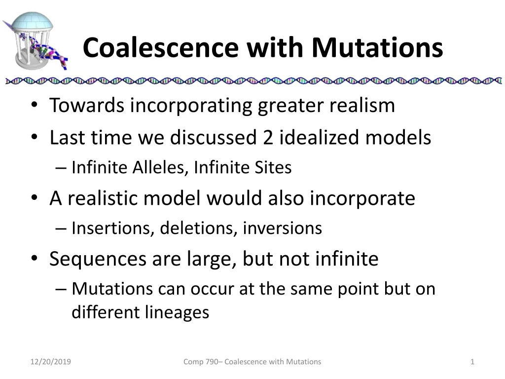
Coalescence with Mutations. Towards incorporating greater realism Last time we discussed 2 idealized models Infinite Alleles, Infinite Sites A realistic model would also incorporate Insertions, deletions, inversions Sequences are large, but not infinite

E N D
Coalescence with Mutations • Towards incorporating greater realism • Last time we discussed 2 idealized models • Infinite Alleles, Infinite Sites • A realistic model would also incorporate • Insertions, deletions, inversions • Sequences are large, but not infinite • Mutations can occur at the same point but on different lineages Comp 790– Coalescence with Mutations
Finite Sites Model • Jukes-Cantor model- all positions are equally likely to mutate, mutations to any of the 3 other nucleotides are equally probable • Kimura model- accommodates that transitions (A<->T and C<->G)occur more frequently than transversions • Positions evolve independently ACCTGCAT ACGTGCAT ACGTGCTT TCCTGCAT ACGTGCTT ACGTGCTA ACGTGCAA TCCTGCAT ACGTGCTT ACGTGCTA ACGTGCAA TCCTGCAT TCCTGCAT Comp 790– Coalescence with Mutations
Wright-Fisher with Mutations • Each gene passed on to the nextgeneration is subject to mutationwith probability u (probability 1 - uit is copied without modification) • Can accommodate any one of InfiniteAlleles, Infinite Sites, or Finite Sites • Overall structure is the same • Working backwards from the present,the probability that a lineage experiencesthe first mutation j generations in the past is: Population of 8 with 4 alleles; one group of 5, and 3 of 1 Comp 790– Coalescence with Mutations
Return of the Basic Coalescent • Formula is similar in form to the discrete coalescent • TM denotes the number of generations until the first mutation event. It is a geometric variable with parameter u. • If time is measured in units of 2N generations then: • Where θ = 4Nu, the population mutation rate, can be interpreted as the expected number of mutations separating two samples Comp 790– Coalescence with Mutations
Probabilities of Events • If we consider n disjoint lineages then the time to the first mutation along any line the distribution is exponential with parameter • Wait for both mutation and coalescence events, then the parameter is the sum of the two parameters (consequence of min(U,V) ~ Exp(a+b)) • Whether the 1st event is a coalescent of mutation event is determined by a biased Bernoulli trials, with probabilities , of mutation for coalescence, and, Comp 790– Coalescence with Mutations
Simulating Sequence Evolution • Simulating a set of genes with mutations • Put k=n, where n is the sample size • Choose an exponential variable with parameter k(k-1+θ)/2 • With probability (k-1)/(k-1+θ) the event is a coalescent event and probability θ/(k-1+θ) it is a mutation event • If a coalescent event, choose a pair randomly to coalesce, set k k-1 • If a mutation event, choose a lineage to mutate • Continue until k is one Comp 790– Coalescence with Mutations
Coalescent in Python • Straightforward translation into Python T = [[i,0.0] for i in xrange(N)] # gene number and time of merge k = N theta = 4.0*N*0.1 t = 0.0 while k > 1: t += expovariate(0.5*k*(k-1+theta)) if (random() < theta/(k-1+theta)): i = randint(0,k-1) T[i] = [T[i], t] else: i = randint(0,k-1) j = randint(0,k-1) while i == j: j = randint(0,k-1) T[i] = [T[i], T[j], t] T.pop(j) k -= 1 Comp 790– Coalescence with Mutations
An Alternate Algorithm • Waiting time until a mutation along a lineage is an exponential distribution with parameter θ/2 (slide 4) • Equivalent to distributing mutations along a t-length path with Poisson distribution having parameter tθ/2 • With mean, tθ/2. • Given the number of mutations on a branch, the times are random • The number and times of mutations on each branch are independent • Thus, coalescence can be computed first, then mutations can be inserted along each branch • The placing mutations on branches is called a “Poisson process” Comp 790– Coalescence with Mutations
Poisson Algorithm • A variant of the continuous-time coalescent with mutations • Simulate the genealogy of N sequences according to a coalescent process with rate (algorithm from lecture 4) • For each branch generate a random number, Mt, using a Poisson distribution with parameter tθ/2, where t is the length of the branch • For each branch, the times of the Mt mutation events are chosen at random Comp 790– Coalescence with Mutations
Benefits of New Algorithm • Mutations can be added onto a genealogy in retrospect • Tweak mutation and coalescent parameters independently • Mutation does not effect the fundamental results of coalescence • Mutations only impact the extant Alleles • How long ago did N haplotypes diverge? • What mutation rate would explain the diversity seen? Comp 790– Coalescence with Mutations
Book • What’s ahead • I will finish chapter 2 next Tuesday • From there on, one of you will be responsible for the a chapter • Each chapter in 2 lectures (pick up the pace a bit), a Thursday followed by a Tuesday • You’ll have a weekend to prepare each lecture • I will do chapter 8 Comp 790– Continuous-Time Coalescence