Download
1 / 13

E N D
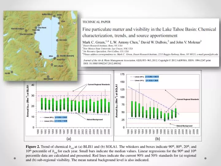
Figure 2. Trend of chemical bextat (a) BLIS1 and (b) SOLA1. The whiskers and boxes indicate 90th, 80th, 20th, and 10th percentile of bextfor each year. Small bars indicate the median values. Linear regressions for the 90th and 10th percentile data are calculated and presented. Red lines indicate the current 90% and 50% standards for (a) regional and (b) sub-regional visibility. The mean natural background level is also indicated.
Spatial Variation Assessed By Satellite • AOD- column-total aerosol light extinction: • AOD = ∫bext(dz) If all aerosol is in boundary layer AOD approximated by bext·L (L=boundary layer depth) • NASA MODIS AOD (Level II) data from Satellites Terra and Aqua • 10 km 10 km resolution at nadir view • Twice daily scans during day time (about 11:00 AM and 1:00 PM • Less valid AOD data available in winter due to frequent cloudy skies over the Lake Tahoe basin • Spatial distribution of AOD is calculated based on valid AOD data points
Assumptions for surface/satellite comparability Spatial homogeneity across pixels and within mixed layers Cloudless sky Temporal correspondence between surface and satellite estimates Constant aerosol extinction properties (e.g., size, composition, and shape)
Domain of Study • 11 11 points in the domain of interest • Surface chemical visibility measurements were made at BLIS and SOLA
Resources http://modis-atmos.gsfc.nasa.gov/MOD04_L2/acquiring.html HDF Viewer Matlabhdfread
AOD Data Interpolation MODIS (Aqua Level 2) AOD data for (a) the western U.S. and (b) Lake Tahoe region on 6/27/2007. Blanks indicate missing or invalid pixels
AOD versus Surface bext(Mm-1) All concurrent data for BLIS from 2007 to 2009
How many % differs from BLIS? • So BLIS represents a very large area (for July 2007)
Average July AOD 2007 2008 2009
Average October AOD 2007 2008 2009
Episodic Aerosol Optical Depth AOD map during the Angora Fire event
Spatial Analysis suggests that: 1) background PM and bext levels are pretty uniform across the Tahoe basin, except during severe wildfire events, 2) influences such as traffic and residential wood combustion are confined in urban “neighborhoods” (sub-pixel), and 3) visibility within the basin would be well bounded by BLIS1 (background) and SOLA1 (maximum) measurements