Download
1 / 43
440 likes | 630 Views
2.7 fs. Generation of short pulses. Ultrashort pulse generation. 15 fs pulse. Single cycle pulse. Time [fs]. Time [fs]. Wavelength [m]. Wavelength [m]. Output pulse of second process as input to a third process. Output pulse of third process as input to a fourth process.

E N D
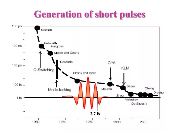
2.7 fs Generation of short pulses
Ultrashort pulse generation 15 fs pulse Single cycle pulse Time [fs] Time [fs] Wavelength [m] Wavelength [m]
Output pulse of second process as input to a third process Output pulse of third process as input to a fourthprocess Output pulse as input to a second process frequency Raman scattering and attosecond pulses Input two frequencies nearly resonant with a Raman resonance. At high intensity, the process cascades many times. Etc. Input pulses 1 0 Raman processes can cascade many times, yielding a series of equally spaced modes =1+/- n0 S. E. Harris and A. V. Sokolov PRL 81, 2894
Dwba= 2994 cm-1 Cascaded Raman generation A. V. Sokolov et al. PRL 85, 85 562 This can be done with nanosecond laser pulses!
Experimental demonstration of cascaded Raman scattering Detuning from 2-photon resonance 2994 cm-1 - 400MHz + 100MHz + 700MHz 75,000 cm-1 (2.3 x 10¹⁵ Hz) of bandwidth has been created! A. V. Sokolov et al. PRL 85, 562
Experimental demonstration of cascaded Raman scattering The different frequencies are locked Pulses with 1 fs duration are measured The spectrum is discrete: the pulses are emitted in a pulse train, separated by the vibrational period. The main advantage of this process: high efficiency The main drawback: the carrier frequency is in the visible regime We cannot produce an isolated pulse. A. V. Sokolov et al. PRL 85, 562
Breaking the femtosecond limit 2001: First observation of an attosecond pulse (650 as) M. Hentschel et al., Nature414, 509-513 (2001) G. Sansone et al., Science314, 443 (2006) 2006: (130 as)
Our main tool: intense laser pulses Field Intensity: 1014 –1015 W/cm2 2.7 fs The force is comparable to the force binding the electrons in the atom or molecule.
With I~1014 W/cm2 Fundamental frequency Attosecond pulse generation process Re-collision Acceleration by the electric field E>100eV Tunnel ionization
Attosecond pulse generation process Acceleration by the electric field Tunnel ionization Optical radiation with attoseconds duration
Attosecond pulse generation process Classical model
Attosecond pulse generation process Classical model
Attosecond pulse generation process Classical model The return times are determined such that x0(t,t0)=0 Long trajectories Short trajectories Ek is the instantaneous frequency of the attosecond pulse
Attosecond pulse generation process Quantum model The electron’s wavefunction The induced dipole moment The dynamics of the free electron is mapped into the optical field
Electron wave packet dynamic Attosecond pulse
Electron wave packet dynamic XUV field: Husimi reprsentation
where only the gas was changed in between. 0,0 0,1 0,2 0,3 0,4 0,5 0,01 0,1 1 H21 Ar N2 normalized signal at H21 el Attosecond pulse generation process Classical model Elliptically polarized light: The electron is shifted in the lateral direction: the recollision probability reduces significantly
Isolating a single attosecond pulse The multi-cycle regime
Isolating a single attosecond pulse The multi-cycle regime Femtosecond pulse 20 fs, 800nm High harmonics I~1014 W/cm2 H15 23.3eV H21 32.6eV H27 41.9eV H39 60.5eV
Attosecond pulse generation process M. Hentschel et al., Nature414, 509-513 (2001)
Attosecond pulse generation process G. Sansone et al., Science314, 443 (2006)
Time resolved measurements in the attosecond regime Attosecond pulses generation Measurement
How to measure an attosecond pulse? XUV Autocorrelation NLO effects:2-photon absorption 2-photon ionization t Problems:low XUV fluxsmall sabs focusing NL Kobayashi et al., Opt. Lett. 23, 64 (1998)
Attosecond streak camera momentum Laser field Photo-electrons Electron release time Attosecond pulse M. Hentschel et al., Nature414, 509-513 (2001)
Momentum transfer depends on instant of electron release within the wave cycle
Mapping time to momentum Momentum change along the EL vector 800-nm laser electric field Δp(t7) Δp(t6) Δp(t5) t1 t2 t3 t4 t5 t6 t7 Δp(t4) instant of electron release Δp(t3) Δp(t2) Δpi Δp(t1) Incident X-ray intensity 0 500 as -500 as Optical-field-driven streak camera J. Itatani et al., Phys. Rev. Lett.88, 173903 (2002) M. Kitzler et al., Phys. Rev. Lett.88, 173904 (2002)
Reconstructed temporal intensity profile and chirp of the xuv excitation pulse: 2 1 1 0 t = 250as xuv Intensity [arb. u.] Instantaneous energy shift [eV] -1 -2 0 -3 -0.4 -0.2 0.0 0.2 -0.4 Time [fs] Full characterization of a sub-fs, ~100-eV XUV pulse Field-free spectrum td = -T0/4 td = +T0/4 = 250 attoseconds!!
Energy shift of sub-fs electron wave-packet ΔW +10 eV 0 -10 eV As we vary the relative delay between the XUV pulse and the 800-nm field, the direction of the emitted electron packet will vary. tD dN/dW
Attosecond streak camera trace 90 80 70 Photoelectron kinetic energy [eV] 60 50 0 2 4 6 8 10 12 14 16 18 20 22 Delay Dt [fs] E. Goulielmakis et al., Science 305, 1267(2004)
RABITT (Reconstruction of Attosecond Beating by Interference of Two-photon Transition) The different paths interfere with a relative phase of: Two photon transition Narrow one photon transition
RABITT (Reconstruction of Attosecond Beating by Interference of Two-photon Transition) RABBITT takes advantage of the interference of the even-harmonic sidebands created when the XUV pulse interacts with the intense IR laser pulse.
Time resolved measurements Can we performed an attosecond pump probe measurement? The main problem is the low photon flax t focusing NL One solution is to use the strong IR field as either the pump or the probe
Core level ionization Auger Decay Attosecond streaking spectroscopy Valence level ionization M. Drescher et al, Nature 419, 803 (2002)
Oscillating dipole The attosecond pulses contains the spatial information of the ground and the free electron wavefunctions.
Imaging the ground state The free electron act as a probe - the re-collision step maps the ground state wave function to the spectrum c ~1A d(t)= a(k) <g|er|eikx-()t>
Harmonic intensities Harmonic intensities from N2 at different molecular angles EL
Reconstructed Molecular Orbital - N2 Reconstructed orbital Calculated orbital J. Itatani, et al., Nature432, 867 (2004).