Understanding Production and Cost Behavior in Property and Construction

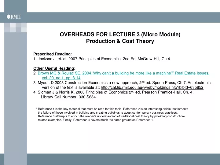
1. Prescribed Reading: 1. Jackson J. et. al. 2007 Principles of Economics, 2nd Ed. McGraw-Hill, Ch 4 Other Useful Reading: 2. Brown MG & Roulac SE, 2004 ‘Why can’t a building be more like a machine?’ Real Estate Issues, vol. 29, no 1, pp. 8-14 3. Myers, D 2008 Construction Economics a new approach, 2nd ed. Spoon Press, Ch 7. An electronic version of the text is available at: http://cat.lib.rmit.edu.au/vwebv/holdingsInfo?bibId=635852 4. Sloman J & Norris K, 2008 Principles of Economics 2nd ed, Pearson Prentice-Hall, Ch. 4, Library Call Number:330 S634 OVERHEADS FOR LECTURE 3 (Micro Module)Production & Cost Theory * Reference 1 is the key material that must be read for this topic. Reference 2 is an interesting article that laments the failure of those involved in building and creating buildings to adopt contemporary business practices. Reference 3 attempts to enrich the reader’s understanding of traditional cost theory by providing construction-related examples. Finally, Reference 4 covers much the same ground as Reference 1.

2. Learning Objectives • This lecture: • Will demonstrate why an understanding of production and cost theory is important for decision-makers in the property and construction sectors • Will describe the behaviour of production and costs (in the short and long-run) • Will examine how to arrive at the cost minimizing input combination for the production of a given output level. Property Economics (Micro - Topic # 3)

3. Why is production & cost behaviour important to understand? A very important reason for property and construction firms to be interested in the behaviour of production and costs is because profit is functionally related to costs P (Profit) = TR (Total Revenue) - TC (Total Cost) Examined last topic Examined this topic and production behaviour (along with technology) will impact on cost. Property Economics (Micro - Topic # 3)

4. The Production Function The Production Function is defined as the relationship between different combinations of inputs and the resultant output An example of a production function that is applicable to rural property is provided below: output of corn Land (hectares) Labour (man years) The inputs are man-years of labour (L) and hectares of land (A) and the output is corn measured in bushels per year. Property Economics (Micro - Topic # 3)

5. The Production Function Continued Illustration: Suppose that 2 man-years (L = 2) is applied to 1 hectare (A = 1) then this will yield annual corn output Q amounting to 200 bushels: Tabular representation of a production function with 2 inputs Property Economics (Micro - Topic # 3)

6. Concepts of Time and Technological Change Short-Run: This is a period when at least one factor of production (input) is fixed Long-Run: This is a period when all factors are variable. Note that the long-run is not sufficiently long for technological change to occur. A technological change will actually alter the relationship between inputs and output. This is said to occur in the very long run. Example of technological Change: Property Economics (Micro - Topic # 3)

7. Short-Run Production Consider the construction of a shopping centre car park where the variable input is labour (L) measured in man-days and the fixed input is the number of cement mixers (K). Then daily output Q measured in square metres of concreted area for different combinations of (K,L) is provided in the following table: Tabular representation of a production function when all inputs are variable Property Economics (Micro - Topic # 3)

8. Short-Run Production Continued Assume in the short run, K is fixed at 2 cement mixers, then only the shaded row of (K, L) combinations apply in the short run* * In this example other raw materials like cement are ignored because our producers have been sub-contracted to use the cement, water and other inputs (eg concreting tools) provided by the main contractor. All the sub-contractors have to do (i.e. the concreters) is provide the labour to lay the concrete as well as prepare the cement in the two cement mixers that they have hired on a daily basis. Property Economics (Micro - Topic # 3)

9. Short-Run Production Continued From the elements of the shaded row (below left) we may pair Q against L to see how Q varies with L holding K fixed at 2 cement mixers (see below right). The short-run production schedule The elements of this shaded row indicate how output Q changes as L changes holding K constant at 2 Property Economics (Micro - Topic # 3)

10. Short-Run Production Continued The data residing in the short-run production schedule (see below left) may be graphed as the short-run production function (see below right) or total product curve. Q: daily concreted area (in m2) The short-run production function L: man-days Property Economics (Micro - Topic # 3)

11. The concept of average product Average Product: Sometimes referred to as the average physical product, the average product (AP) of an input (say labour) is defined as the average contribution of each unit of the variable input to output. AP = output /input level where: “input level” = the number of units of a particular input applied to production As an illustration of the concept of average product let us compute the average product of labour from the previously generated short-run production schedule. Property Economics (Micro - Topic # 3)

12. Illustration of the average product concept Recall that: AP = output / input level Thus, when L = 4 man-days, Q = 280 m2 and so the average product of labour (APL) is given by: APL = output / labour input = Q/L = 280/4 = 70 In other words, when 4 man days are applied to the production process each man-day is contributing 70 m2 of laid concrete per day. Note: the average product of an input varies with the level of the input applied to production. This may be seen from the adjacent schedule on this page. The behaviour of AP may also be gauged by graphing AP against the input level. Such a graph is called the average product curve. Property Economics (Micro - Topic # 3)

13. The Average Product Curve (charting average product against the input level) For our example we obtain the average product curve for labour by plotting APL (on vertical axis) against L (on horizontal axis) The average product curve Q/L: average product of labour L: Labour (man-days) Property Economics (Micro - Topic # 3)

14. The Concept of Marginal Product Marginal Product: Sometimes referred to as the marginal physical product, the marginal product (MP) of an input (say labour) is defined as the change in output per unit change in that input all other inputs held constant. MP = output / input where: input = 1 As an illustration of the concept of marginal product let us compute the marginal product of labour from the previously generated short-run production schedule. Property Economics (Micro - Topic # 3)

15. Illustration of the Marginal Product Concept Recall that: MP = output / input where: input = 1 Thus, when L increases from 2 to 3 man-days, Q increases from 100 to 200 m2 and so the marginal product of labour (MPL) is given by: MPL = output / input = 100/1= 100 Note: MP varies with the input level. For instance, between and L=0 and L=1, MPL = 30 but between an L=3 and L=4, MPL = 80. This tendency for the MP to vary with the input level may also be gauged by graphing MP against the input level. Such a graph is called the marginal product curve. Property Economics (Micro - Topic # 3)

16. The Marginal Product Curve (charting marginal product against the input level) For our example we obtain the marginal product curve for labour by plotting MPL (on vertical axis) against L. (on horizontal axis). Note that the MP values are properly plotted against the midpoints between successive unit increments in the variable input. MPL = Q/L The marginal product curve L: labour (man-days) Property Economics (Micro - Topic # 3)

17. The Law of Diminishing Marginal Returns Re-inspecting the marginal product curve, observe that marginal product begins to fall at some point. This phenomenon is referred to as the Law of diminishing marginal returns. Simply stated the law says: As the variable input is increased a unit at a time (holding constant all other inputs), a point will be reached where output will only increase by decreasing amounts. MPL = Q/L The marginal product curve diminishing returns set in beyond this point L: labour (man-days) Property Economics (Micro - Topic # 3)

18. Relationships among TP, MP and AP AP rises (falls) when MP>AP (MP<AP) AP is at a maximum when MP = AP TP rises (falls) when MP > 0 (MP < 0) TP is at a maximum when MP = 0 The law of diminishing marginal returns is responsible for the inverted U-shape of both the MP and AP curves When MP reaches its maximum and begins to descend, the law of diminishing marginal returns comes into force. This will be at the point where there is an inflexion point on the TP curve TP, MPL , APL TP inflexion point on TP curve appears here APL L MPL Property Economics (Micro - Topic # 3)

19. The Stages of Production Stage 1: Increasing Returns to the Variable Factor As L rises, TP rises, MP or AP or both rise Stage 2: Diminishing Returns to the Variable Factor As L rises, TP is rising but MP and AP are both falling. Stage 3: Decreasing Returns to the Variable Factor As L rises, TP is falling, MP and AP are both falling and MP is negative. It may be shown (but not here) that firms prefer to produce in Stage 2 as in Stage 1 (3) there is under (over) utilisation of fixed inputs TP, MPL , APL TP Stage 1 Stage 2 Stage 3 APL L MPL Property Economics (Micro - Topic # 3)

20. Preliminary Cost Concepts What exactly do we mean by production costs? ANSWER: private opportunity costs of production (or construction) The emphasis on PRIVATE is an important one The profit maximizing firm is generally assumed to be only concerned with the costs it privately bears in the course of its production activity. There is absolutely no assurance that the full social costs of production are considered by a firm. This will only the case if the firm is required to internalize such costs by government or if a truly socially conscious firm decides to do so on its own accord. Property Economics (Micro - Topic # 3)

21. Preliminary Cost Concepts Continued Private Opportunity Costs Continued The emphasis on OPPORTUNITY COSTS is an important one. Opportunity Costs comprise: Explicit Costs: These are those associated with an observable outflow of money when the firm purchases inputs for production activity. Implicit Costs: These include the dollar imputed opportunity costs of all self owned resources. Implicit costs also include other costs like depreciation expenses that are not directly associated with an explicitly observable outflow of money. Accountants recognize explicit costs and some implicit costs like depreciation. However, unlike economists they are not typically concerned with the opportunity costs of self-owned resources. Property Economics (Micro - Topic # 3)

22. Preliminary Cost Concepts Continued Private Opportunity Costs Continued Example: Dan is a sole trader who specializes in house restorations. He owns his own utility as well as an office two blocks away from home. At the back of the office is big yard where Dan has a large stock of second hand construction material that he has amassed virtually at zero cost from home wreckage sites. He is currently considering undertaking a house restoration opportunity that will occupy him for the best part of the year. The opportunity cost of using old tiles and clinker bricks stored in the yard for the project is the forgone opportunity of selling them on the open market. The opportunity cost of the utility truck is the lost opportunity of not leasing it out to somebody else. There is also the opportunity cost associated with the salary that he forgoes by not working for someone else if he occupies himself with the house restoration. Property Economics (Micro - Topic # 3)

23. Preliminary Cost Concepts Continued Short-Run Cost Behaviour It will be recalled that the short run is a period when at least one input is fixed whilst some inputs are variable. In the short-run we distinguish between costs associated with fixed inputs and those which are associated with variable inputs. Fixed Costs: are costs associated with fixed inputs. These costs are borne by the firm whether it produces or not Variable Costs:are costs associated with variable inputs. These costs will vary with output because in the short-run, variations in output can only arise from variations in the variable inputs. Property Economics (Micro - Topic # 3)

24. Preliminary Cost Concepts Continued • Examples of Variable Costs in Construction • The cost of using more or less • - labour • construction material • - site management • construction equipment (in terms of wear and tear if it is self owned) or rental costs (if it is leased) • will vary with the amount of construction activity that is undertaken by the firm per period. Property Economics (Micro - Topic # 3)

25. Preliminary Cost Concepts Continued • Examples of Fixed Costs in Construction • Whether construction takes place or not over a short period some costs borne by the firm will remain fixed (or invariant). Examples would include: • - work-cover insurance, salaries and superannuation premia for permanent staff • insurance cover for office building and contents, tools, utility trucks etc. • property rates, water and energy bills at the head office • an adequate normal return to keep the firm’s owners in the construction industry • interest on funds borrowed in previous periods to fund the procurement of construction materials or capital expansion. • rent forgone by not leasing out self-owned construction equipment and tools Property Economics (Micro - Topic # 3)

26. Preliminary Cost Concepts Continued Construction Costs in the Real World Download at this link a spreadsheet that compares costs of different types of construction service firms produced by the Australian Bureau of Statistics. Property Economics (Micro - Topic # 3)

27. Short-Run Total Costs Costs are determined by the price and quantities of inputs used in the production (construction) process We shall assume that all factor prices facing the firm (whether explicit or implicit) are constant - that is the firm is too small or has insufficient market power to influence the purchase price of inputs. Total fixed Costs (TFC) Suppose in our car lot example that the number of concrete mixers K is fixed at 2 (i.e. K=2) and the daily rental charge per concrete mixer is PK = $400. Then: Total Fixed Cost (TFC) = PKK = ($400)2 = $800 Of course if there were other fixed inputs, these would have to be costed and included in the expression for TFC. Property Economics (Micro - Topic # 3)

28. Short-Run Total Costs Continued Total Variable Cost (TVC) Let L denote the variable number of man-days that are hired per day and assume that the daily price (or wage) per man-day is PL= $300. Then the expression for TVC would be given by: Total Variable Cost (TVC) = PLL= $300L Of course, if there were other “price times variable input” terms like: PLL, these would also have to be included in the expression for TVC. Total Cost (TC) Is defined as the sum of TFC and TVC. In other words: TC = TFC + TVC = PKK + PLL = $400(2) + $300L = $800 + $300L Property Economics (Micro - Topic # 3)

29. Short-Run Total Costs Continued Short-Run Total Cost Schedules The following table demonstrates numerically how TFC, TVC and TC behave at different output levels (and indirectly the variable input). In the adjacent table each of the total cost measures may be graphed against output to arrive at the short-run total cost curves. Property Economics (Micro - Topic # 3)

30. Short-Run Total Costs Continued Short-Run Total Cost Curves Graphing TC, TFC and TVC in the table (below left) against Q we obtain the TC, TFC and TVC curves. These curves are pictorial representations of how each measure of total cost varies with output. $ TC TVC TFC Q Property Economics (Micro - Topic # 3)

31. Short-Run Total Costs Continued The Relationship among Short-Run Total Cost Curves The vertical distance between TC and TVC at any given output level will equal TFC. The Law of Increasing Costs The law of increasing costs which is the counterpart of the law of diminishing returns states that: As output increases one unit at a time, eventually a point will be reached where cost increases by increasing amounts. In our example this occurs when Q = 200. This is the output level vertically beneath the inflexion point on either the TVC or TC curves $ TC Inflexion points beyond which the law of increasing costs manifests itself TVC TFC = 800 TFC TFC = 800 Q Property Economics (Micro - Topic # 3)

32. Short-Run Average Costs Continued Often it is preferable to examine the behaviour of short-run average costs rather than total costs as the former are more comparable with average revenue or price. From the previous discussion of short-run total costs recall that: TC = TFC + TVC Dividing through this expression by Q we obtain: TC/Q = TFC/Q + TVC/Q or ATC = AFC + AVC AVC (average variable cost) AFC (average fixed cost) ATC (short-run average total cost) Property Economics (Micro - Topic # 3)

33. Short-Run Average Costs Continued The Short Run Average Cost Schedules In the shaded columns of the following table find the schedules for AFC, AVC and ATC.The entries in these schedules have been derived according to the following definitions: AFC = TFC/Q; AVC = TVC/Q and ATC = AFC + AVC or TC/Q These schedules show tabularly how AFC, AVC and ATC behave as output varies. A better appreciation of their behaviour may be portrayed in the form of short-run average cost curves. Property Economics (Micro - Topic # 3)

34. Short-Run Average Costs Continued The Short Run Average Cost Curves We may graph the data for AFC, AVC and ATC schedules (see table below) as the AFC, AVC and ATC cost curves (appearing in the adjacent graph). $/unit ATC AVC AFC Q Property Economics (Micro - Topic # 3)

35. Short-Run Average Costs Continued The Short Run Average Cost Curves Continued Shape of AFC Curve AFC is a geometrically decaying function of Q Shape of AVC Curve AVC first declines with output but eventually rises as a result of the law of increasing costs or diminishing marginal returns Generally the AVC curve will be U-shaped $/unit ATC AVC AFC Q Property Economics (Micro - Topic # 3)

36. Short-Run Average Costs Continued The Short Run Average Cost Curves Continued Shape of ATC Curve At any given output level, the ATC curve is the vertical summation of the AFC and AVC curves. That is the gap between ATC and AVC equals AFC at any given output level. Generally it is the case that the ATC curve is U-shaped like the AVC curve. Normally the ATC reaches its minimum at a higher output level than AVC because for a while the rise in AVC is more than outweighed by the fall in AFC $/unit ATC AVC AFC Q Property Economics (Micro - Topic # 3)

37. Short-Run Marginal Cost Short Run Marginal Cost (MC) is defined as the increase (decrease) in cost if the firm increases (decreases) output by one unit in the short-run. This definition may be expressed algebraically: MC = TC/Q where Q = 1 Note: Since TFC does not change in the short-run, the only source of change in TC may arise when TVC changes. Hence the preceding expression may also be rewritten as: MC = TVC/Q = where Q = 1 Example: Suppose that currently a large residential building company is constructing 5 homes of a particular design per 2 months (which we shall take as the short-run). Let us also assume that it can construct these homes at a total cost of $1,200,000. If instead the firm were to produce a total of 6 homes at a total cost of $1,450,000. Then: TVC = TC = $250,000 and MC = TVC/Q = DTC/DQ = $250,000/1 = $250,000 Property Economics (Micro - Topic # 3)

38. Short-Run Marginal Cost Continued Short Run Marginal Cost (MC) Continued As with the short-run average cost curves discussed earlier it is possible to examine the behaviour of MC by inspecting the entries for MC in an appropriate schedule or a chart of MC plotted against Q. To generate the MC schedule , a schedule for TC or TVC is required with output Q increasing 1 unit at a time. However, the schedules for TC and TVC used in our running example (see adjacent table) have NOT been constructed with Q increasing in unit increments. If however, the TVC (TC) curve is linear between any two successive output levels in this table, MC will be constant for each unit in this output range. This is because: MC = TVC/Q = TC/Q will measure the constant slope of the linear segment of the TVC (TC) curve between two such successive output levels. Property Economics (Micro - Topic # 3)

39. Short-Run Marginal Cost Continued The Short Run Marginal Cost (MC) Schedule Under the assumption that the TVC (TC) curve comprises differently sloped linear segments over successive output ranges, a schedule for MC has been prepared directly below: Property Economics (Micro - Topic # 3)

40. Short-Run Marginal Cost Continued The Short Run Marginal Cost (MC) Curve It will be recalled that when the MP curve was charted, the measures of marginal product were plotted at the midpoints of each unit increment of the variable input. An analogous procedure applies for the plotting of marginal cost measures except that they are plotted against the midpoint of successive unit increments in output. In the adjacent graph the resultant MC curve has been superimposed onto the previously generated short-run average cost curves $/unit MC ATC AVC AFC Q Property Economics (Micro - Topic # 3)

41. Short-Run Marginal Cost Continued The Short Run Marginal Cost (MC) Curve Continued There are important relationships among MC, AVC and ATC. When: MC > ATC (AVC), then ATC (AVC) is rising MC < ATC (AVC), then ATC (AVC) is falling MC = ATC (AVC) then ATC (AVC) is at a minimum. We shall see in a subsequent topic that knowledge of MC is important when it comes to determining the profit maximizing output level . $/unit MC ATC AVC AFC Q Property Economics (Micro - Topic # 3)

42. Long-Run Costs The Long Run Average Costs Curve Consider a manufacturer of domestic air-conditioners. Currently, the manufacturer is considering several plant extension options : A, B or C for its existing factory. In the following diagram, the firm’s short run average cost curve is given by SRATC*. The short-run cost curves for alternative plant extension options: SRATCA, SRATCB and SRATCC also appear in this diagram. $/unit SRATC* SRATCA SRATCB SRATCC Q Property Economics (Micro - Topic # 3)

43. Long-Run Costs Continued The Long Run Average Costs Curve Continued In the long run, all inputs are variable including the size of the factory. So the manufacturer should be mindful that the existing plant size may not be the most economical one to operate over the long-run. For instance, if demand for air-conditioners is expected to be Q* per period over the long run, then the existing plant size should be extended from its current size to the one implied by Option A because the unit cost of production will be CA rather than C*. $/unit SRATC* (Existing Plant Size) SRATCA SRATCB C* SRATCC CA Q Q* Property Economics (Micro - Topic # 3)

44. Long-Run Costs Continued The Long Run Average Costs Curve More generally if it is expected that : Q* < Q1 then the existing plant size should be retained Q1 < Q* < Q2 then the option A extension is justified Q2 < Q* < Q3 then the option B extension is justified Q3 < Q* then option C extension is justified $/unit SRATC* SRATCA SRATCB SRATCC p q r Q Q1 Q2 Q3 Property Economics (Micro - Topic # 3)

45. Long-Run Costs Continued The Long Run Average Cost Curve (LRATC) Continued The long run average total cost curve shows the minimum average cost of producing output Q when plant size may be varied over the long-run. In our example LRATC is given by the scalloped shaped line graph marked with crosses that passes through points p, q and r. $/unit SRATC* X SRATCA X SRATCB X X SRATCC p X X q X X X r X X X X Q Q1 Q2 Q3 Property Economics (Micro - Topic # 3)

46. Long-Run Costs Continued The Long Run Average Cost Curve Continued If there were an infinite number of plant sizes (or for that matter plant extension options) the long run average cost curve (LRAC) would be the envelope curve of the associated short-run average cost curves: SRATCA, SRATCB , ..... SRATCJ .... SRATCN . LRATC $/unit SRATCA SRATCB SRATCN SRATCJ Q Property Economics (Micro - Topic # 3)

47. Long-Run Costs Continued The Long Run Average Cost Curve Continued The LRAC curve is depicted as a U-shaped curve in most text books. The declining section of the LRATC depicts the phenomenon of Internal economies of scale or savings (falling unit costs) that arise due to the increases in plant size and output. Eventually the curve begins to rise due to the phenomenon of internal diseconomies of scale. LRATC $/unit internal economies of scale internal diseconomies of scale Q Property Economics (Micro - Topic # 3)

48. Long-Run Costs Continued The Long Run Average Cost Curve Continued Internal economies (diseconomies) of scale arise when there are increasing (decreasing) returns to scale in production. Increasing (decreasing) returns to scale arises when production increases by a greater (smaller) percentage than an equi-proportionate change in all inputs. LRATC $/unit increasing returns to scale decreasing returns to scale Q Property Economics (Micro - Topic # 3)

49. Long-Run Costs Continued The Long Run Average Cost Curve Continued Sometimes the LRATC flattens out as indicated below. This is attributable to a phenomenon known as constant returns to scale. Constant returns to scale arises when production increases by the same percentage as an equi-proportionate increase in all inputs. $/unit LRATC The horizontal section of LRATC is due to constant returns to scale Q Property Economics (Micro - Topic # 3)

50. Long-Run Costs Continued • Internal Economies of Scale • As previously mentioned, these are the savings that arise from a larger plant size and output. Internal economies may be categorized under two main headings: • Real Economies: • opportunities for specialization and division of managerial as well as labour tasks • opportunities for using more efficient larger capacity equipment • savings arising from the more economical utilization of plant and equipment • opportunities for spreading the fixed costs of overhead processes over a larger output level. • the container principle (output is related to volume but cost is related to surface area) • the larger is production, the easier it is to produce by-products from waste • Pecuniary Economies: • When the firm is very large it is able to reap savings because it is able to bulk purchase its productive factors. For example it may be able to: • procure lower interest rates and better credit terms • negotiate bulk purchase discounts for its raw materials as well as lower freight charges • to force wages down if it is a very large employer Property Economics (Micro - Topic # 3)