Download
1 / 45
450 likes | 456 Views
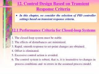
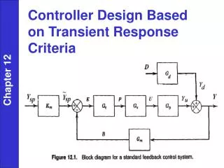
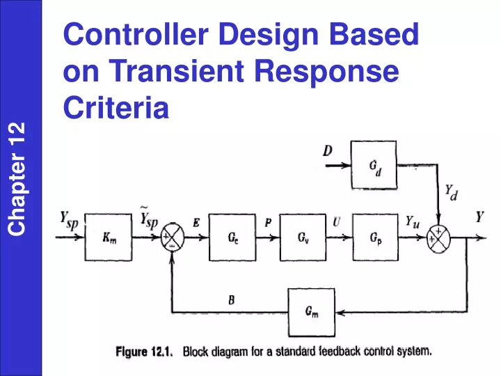
Controller Design Based on Transient Response Criteria. Chapter 12. Desirable Controller Features 0. Stable 1. Quick responding 2. Adequate disturbance rejection 3. Insensitive to model, measurement errors 4. Avoids excessive controller action

E N D
Controller Design Based on Transient Response Criteria Chapter 12
Desirable Controller Features 0. Stable 1. Quick responding 2. Adequate disturbance rejection 3. Insensitive to model, measurement errors 4. Avoids excessive controller action 5. Suitable over a wide range of operating conditions Impossible to satisfy all 5 unless self-tuning. Use “optimum sloppiness" Chapter 12
Alternatives for Controller Design 1.Tuning correlations – most limited to 1st order plus dead time 2.Closed-loop transfer function - analysis of stability or response characteristics. 3.Repetitive simulation (requires computer software like MATLAB and Simulink) 4.Frequency response - stability and performance (requires computer simulation and graphics) 5.On-line controller cycling (field tuning) Chapter 12
Controller Synthesis - Time Domain Time-domain techniques can be classified into two groups: (a) Criteria based on a few points in the response (b) Criteria based on the entire response, or integral criteria Approach (a): settling time, % overshoot, rise time, decay ratio (Fig. 5.10 can be viewed as closed-loop response) Chapter 12 Process model Several methods based on 1/4 decay ratio have been proposed: Cohen-Coon, Ziegler-Nichols
Approach (b) 1. Integral of square error (ISE) 2. Integral of absolute value of error (IAE) 3. Time-weighted IAE Pick controller parameters to minimize integral. IAE allows larger deviation than ISE (smaller overshoots) ISE longer settling time ITAE weights errors occurring later more heavily Approximate optimum tuning parameters are correlated with K, , (Table 12.3). Chapter 12
Summary of Tuning Relationships • 1. KCis inversely proportional to KPKVKM . • 2. KC decreases as / increases. • 3. I and D increase as / increases (typically D = 0.25 I ). • 4. Reduce Kc, when adding more integral action; increase Kc, when adding derivative action • 5. To reduce oscillation, decrease KC and increase I . Chapter 12
Disadvantages of Tuning Correlations 1. Stability margin is not quantified. 2. Control laws can be vendor - specific. 3. First order + time delay model can be inaccurate. 4. Kp, t, and θcan vary. 5. Resolution, measurement errors decrease stability margins. 6. ¼ decay ratio not conservative standard (too oscillatory). Chapter 12
Example: Second Order Process with PI Controller Can Yield Second Order Closed-loop Response Chapter 12 or PI: LettI = t1,wheret1 > t2 Canceling terms, Check gain (s = 0)
2nd order response with... and Select Kc to give (overshoot) Chapter 12 Figure. Step response of underdamped second-order processes and first-order process.
Direct Synthesis ( G includes Gm, Gv) 1. Specify closed-loop response (transfer function) Chapter 12 2. Need process model, (= GPGMGV) 3. Solve for Gc, (12-3b)
Specify Closed – Loop Transfer Function (first – order response, no offset) Chapter 12 But other variations of (12-6) can be used (e.g., replace time delay with polynomial approximation)
Derivation of PI Controller for FOPTD Process Consider the standard first-order-plus-time-delay model, Chapter 12 Specify closed-loop response as FOPTD (12-6), but approximate Substituting and rearranging gives a PI controller, with the following controller settings:
Derivation of PID Controller for FOPTD Process: let (12-3b) Chapter 12 (12-2a) (12-30)
Second-Order-plus-Time-Delay (SOPTD) Model Consider a second-order-plus-time-delay model, Use of FOPTD closed-loop response (12-6) and time delay approximation gives a PID controller in parallel form, Chapter 12 where
Example 12.1 Use the DS design method to calculate PID controller settings for the process: Consider three values of the desired closed-loop time constant: τ = 1, 3, and 10. Evaluate the controllers for unit step changes in both the set point and the disturbance, assuming that Gd = G. Perform the evaluation for two cases: Chapter 12 • The process model is perfect ( = G). • The model gain is = 0.9, instead of the actual value, K = 2. This model error could cause a robustness problem in the controller for K = 2.
The IMC controller settings for this example are: Note only Kc is affected by the change in process gain.
The values of Kc decrease as increases, but the values of and do not change, as indicated by Eq. 12-14. Chapter 12 Figure 12.3 Simulation results for Example 12.1 (a): correct model gain.
Chapter 12 Figure 12.4 Simulation results for Example 12.1 (b): incorrect model gain.
Controller Tuning Relations Model-based design methods such as DS and IMC produce PI or PID controllers for certain classes of process models, with one tuning parameter tc (see Table 12.1) How to Select tc? Chapter 12 • Several IMC guidelines for have been published for the model in Eq. 12-10: • > 0.8 and (Rivera et al., 1986) • (Chien and Fruehauf, 1990) • (Skogestad, 2003)
Tuning for Lag-Dominant Models • First- or second-order models with relatively small time delays are referred to as lag-dominant models. • The IMC and DS methods provide satisfactory set-point responses, but very slow disturbance responses, because the value of is very large. • Fortunately, this problem can be solved in three different ways. • Method 1: Integrator Approximation Chapter 12 • Then can use the IMC tuning rules (Rule M or N) to specify the controller settings.
Method 2. Limit the Value of tI • Skogestad (2003) has proposed limiting the value of : where t1 is the largest time constant (if there are two). Chapter 12 Method 3. Design the Controller for Disturbances, Rather Set-point Changes • The desired CLTF is expressed in terms of (Y/D)d, rather than (Y/Ysp)d • Reference: Chen & Seborg (2002)
Example 12.4 Consider a lag-dominant model with Chapter 12 Design three PI controllers: • IMC • IMC based on the integrator approximation in Eq. 12-33 • IMC with Skogestad’s modification (Eq. 12-34)
Evaluate the three controllers by comparing their performance for unit step changes in both set point and disturbance. Assume that the model is perfect and that Gd(s) = G(s). Solution The PI controller settings are: Chapter 12
Figure 12.8. Comparison of set-point responses (top) and disturbance responses (bottom) for Example 12.4. The responses for the integrator approximation and Chen and Seborg (discussed in textbook) methods are essentially identical. Chapter 12
On-Line Controller Tuning • Controller tuning inevitably involves a tradeoff between performance and robustness. • Controller settings do not have to be precisely determined. In general, a small change in a controller setting from its best value (for example, ±10%) has little effect on closed-loop responses. • For most plants, it is not feasible to manually tune each controller. Tuning is usually done by a control specialist (engineer or technician) or by a plant operator. Because each person is typically responsible for 300 to 1000 control loops, it is not feasible to tune every controller. • Diagnostic techniques for monitoring control system performance are available. Chapter 12
Controller Tuning and Troubleshooting Control Loops Chapter 12
Ziegler-Nichols Rules: These well-known tuning rules were published by Z-N in 1942: Chapter 12 Z-N controller settings are widely considered to be an "industry standard". Z-N settings were developed to provide 1/4 decay ratio -- too oscillatory?
Modified Z-N settings for PID control Chapter 12
Chapter 12 Figure 12.15 Typical process reaction curves: (a) non-self-regulating process, (b) self-regulating process.
Chapter 12 Figure 12.16 Process reaction curve for Example 12.8.
Chapter 12 Figure 12.17 Block diagram for Example 12.8.
Chapter 12 Previous chapter Next chapter