Download
1 / 20
200 likes | 335 Views
Kinetics II. Lecture 15 . Rates and Concentrations. Knowing the rate constant (usually empirically determined), we can compute rate. Integrating rate of first order reaction gives: Graph shows how CO 2 concentration changes in the reaction CO 2 + H 2 O = H 2 CO 3.

E N D
Kinetics II Lecture 15
Rates and Concentrations • Knowing the rate constant (usually empirically determined), we can compute rate. • Integrating rate of first order reaction gives: • Graph shows how CO2 concentration changes in the reaction CO2 + H2O = H2CO3
Elementary or Not? • Can’t always predict whether a reaction is elementary or not just by looking at it. The earlier rules about order of reaction provide a test. • For example, 2NO2 –> 2NO +O2 • Rate of reaction turns out to be • What does does this tell us? • The reaction is elementary.
Elementary or Not? • Now consider 2O3–> 3O2 • Rate of this reaction turns out to be: • Since it depends on the concentration of a reactant, it is not an elementary reaction. • Indeed, it is a fairly complex one involving a reactive intermediate, O˚, which does not appear in the reaction.
Rates of Complex Reactions • Complex reactions that involve a series of steps that must occur in sequence are called chain reactions. • In a chain reaction when one step is much slower than the others, the overall rate will be determined by that step, which is known as the rate-determining step. • Complex reactions can involve alternate routes or branches (read about H2 combustion in book). • In a branch, the rate of the fastest branch will determine that step.
Principle of Detailed Balancing • Consider a reversible reaction such as A = B • The equilibrium condition is k+[A]eq = k–[B]eq • note typo in book: + and - should be subscripted in eqn 5.40 p172. • where k+ and k– are the forward and reverse rate constants, respectively. This is the principle of detailed balancing. • Rearranging we have ? Kapp
Relating k and K • We can write K as: • For constant ∆S: • where C is a constant. • See anything familiar? • Then
Barrier Energies • Our equation was • Its apparent then that: • We can think of the barrier, or activation energy as an energy hill the reaction must climb to reach the valley on the other side. • Energy released by the reaction, ∆Hr, is the depth of the energy valley.
Frequency Factors and Entropies • A similar sort of derivation yields the following • A relates to the frequency of opportunity for reaction (beat of as clock). • This tells us the ratio of frequency factors is exponentially related to the entropy difference, or randomness difference, of the two sides of the reaction. • It can be shown that the frequency factor relates to entropy as: • where ∆S* is the entropy difference between the initial state and the activated state.
Fundamental Frequency • The term • is known as the fundamental frequency • k has units of joules/kelvin, T has units of kelvins, and h has units of sec-1, so the above has units of time (6.21 x 10⁻¹² sec at 298K, or 2.08 x 10⁻¹⁰ T sec).
Reactive Intermediates • Transition state theory supposes that a reaction such as • A + BC –> AC + B • proceeds through formation of an activated complex, ABC*, called a reactive intermediate, such that the reaction mechanism is: A + BC –> ABC* ABC* –> AC + B • The reactive intermediate is supposed to be in equilibrium with both reactants and products, e.g., • Free energy of reaction for formation of complex is:
Predicting reaction rates • Combining these relationships, we have: • Example to the left shows predicted vs. observed reaction rates for the calcite-aragonite transition. • In this case, the above rate is converted to a velocity by multiplying by lattice spacing.
Suppose our reaction A + BC –> AC + B • is reversible. The net rate of reaction is Rnet = R+- R– • If ∆Gr is the free energy difference between products and reactants and ∆G* is free energy difference between reactants and activated complex, then ∆Gr - ∆G* must be difference between activated complex and products. Therefore: • -∆Gris often called the affinity of reaction and sometimes designated Ar(but we won’t). • Then
∆G and Rates • Provided this is an elementary reaction, then the rate may be written as: • Note, activation energy, EA and barrier energy, EB, are the same thing. • In the reaction, the stoichiometric coefficients are 1. • In a system not far from equilibrium, ∆G/RT is small and we may use the approximation ex = 1 + x to obtain: • ∆G is the chemical energy powering the reaction. At equilibrium, ∆G is 0 and the rate of reaction is 0. The further from equilibrium the system is, the more the energy available to power the reaction. Thus the rate will scale with available chemical energy, ∆Gr.
Computing the Reaction Affinity (∆G) • We’ve seen the rate should depend on ∆G, how can we compute it as reaction progresses? • Consider a reaction aA +bB = cC +dD • At equilibrium: • Under non-equilibrium conditions, this equality does not hold. We define the ratio on the right as the reaction quotient: • At equilibrium, ∆G is 0 (and ln K = e–∆G˚/RT) • Under non-equilibrium conditions, ∆G = ∆G˚ + RT ln Q • and ∆G = RT ln Q/K
We expect then that (not far from equilibrium) the reaction should proceed at a rate: • Consider now a reaction that depends on temperature (e.g., α- to β-quartz). Another approach is to remember ∆G = ∆H - T∆S • At equilibrium this is equal to 0. At some non-equilibrium temperature, T, then • ∆G = ∆H - ∆Heq - T∆S+ Teq∆Seq • If we are close to the equilibrium temperature, we may consider ∆H and ∆S constant, to that this becomes: ∆G = -∆T∆S • and also Note: equation incorrect in book.
Rates of Geochemical Reactions Wood and Walther used this equation to compute rates. This figure compares compares observed (symbols) with predicted (line).