Download
1 / 23
230 likes | 282 Views
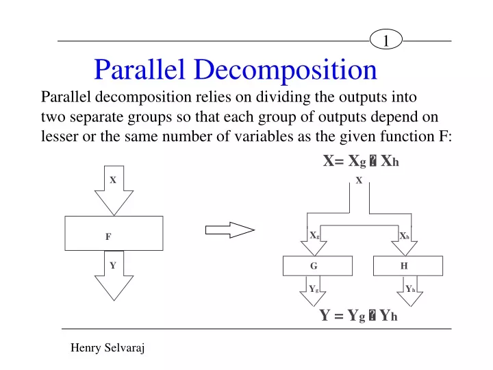
X. X. X g. X h. F. G. H. Y. Y g. Y h. Parallel Decomposition. Parallel decomposition relies on dividing the outputs into two separate groups so that each group of outputs depend on lesser or the same number of variables as the given function F:. X= X g X h. Y = Y g Y h.

E N D
X X Xg Xh F G H Y Yg Yh Parallel Decomposition Parallel decomposition relies on dividing the outputs into two separate groups so that each group of outputs depend on lesser or the same number of variables as the given function F: X= Xg Xh Y = Yg Yh
X 3 5 3 5 9 9 6 X Xg Xh F G H Y Yg Yh Parallel Decomposition X= Xg Xh Y = Yg Yh
Truth table Yh Truth table Yg
Serial decomposition relies on partitioning the input variables in such a way as to obtain a two-level functional dependency F = H(A, G(B C)).
X A X B C G F Y H Y Serial Decomposition
Necessary and sufficient condition for the existence of a serial decomposition There exists a serial decomposition of F if and only if there exists a partition G, such that: (a) G P(B C), and (b) P(A) G PF.
Partition G in the theorem represents function G. In particular,the number of blocks in , , determines the number of output variables of G, log2.
Let A = {x1}, B = {x2,x3,x0}, C = . G = ,.., = (1,4,7,9; 1,2,3,9,11; 0,1,2,7,10,11; 5,6,8). Verify if serial decomposition exists for the given bound set B. P(A) = (0,3,5,7,9,10; 0,1,2,4,6,8,11) P(B) = P0(B),..,P6(B) = (6,8; 0,1,7; 5,6; 0,1,2; 1,4,7,9; 10,11; 1,2,3,9,11) PF = (7,9; 3,4,5,6,8,9; 0,1,2,7,10,11; 1,3,4,5) P(A)·G = (1,4; 7,9; 1,2,11; 3,9; 0,7,10; 0,1,2,11; 5; 6,8) Hence, P(A) · G PF. Thus, according to Theorem, function F is decomposable as F = H(x1,G(x2,x3,x0)), where G is a two-output function.
The main task of decomposition is to verify if a subset of input variables for function G which, when applied as a subfunction to function H will generate the final function F, i.e. to find a P(B), such that there exists G P(B) which satisfies condition a) and b) in the theorem. To solve this problem, consider a subset of input variables B, and an m‑block partition P(B) = (B1; B2 ;...; Bm) generated by this subset.
A relation of compatibility of partition blocks is used to verify whether or not partition P(B) is suitable for serial decomposition. Two blocks Bi,Bj P(B) are compatible if and only if partition obtained from partition P(B) by merging blocks Bi and Bj into a single block Bj satisfies conditions in the decomposition theorem, i.e. if and only if P(A) PF
Compatible class A subset of n partition blocks, B = {Bi1,Bi2,...,Bin}, where Bij P(B), is a class of compatible blocks for partition P(B) if and only if all blocks in B are pairwise compatible.
Maximum Compatible Class A compatible class is called Maximum Compatible Class (MCC) if and only if it cannot be properly covered by any other compatible class.
Let B = {x1,x2,x4} and A = {x3,x5}. Then, PF = (3,10,14,15; 12; 3,16,12,14; 5,7,8,13; 1,8,9,14; 4,8,11,12; 2,6,8,12,14), P(A) = (2,13,14; 5,11; 1,3,7,8,9,15; 4,6,10,12) and P(B) = (14,15; 2,3; 9,11,12; 6; 13; 1; 8,10; 4,5,7)
Let us check if B0 = (14,15) and B2 = (9,11,12) are compatible. We have: P02(B) = (9,11,12,14,15; 2,3; 6; 13; 1; 8,10; 4,5,7) P(A) P02(B) = (2; 13; 14; 5; 11; 1; 3; 7; 8; 9,15; 4; 6; 10; 12), does not satisfy P(A) P02(B) PF, B0 and B2 are not compatible.
For B0 = {14,15} and B1 = {2,3}, we obtain P01(B) = (14,15,2,3; 9,11,12; 6; 13; 1; 8,10; 4,5,7) and P(A) P01(B) = (2,14; 13; 5;11; 1; 3,15; 7; 8; 9; 4; 6; 10; 12) PF. Thus, B0 and B1 are compatible. In a similar way we check the compatibility of each pair of blocks in P(B) finding the following relation COM = {(B0,B1), (B0,B3), (B1,B3), (B2,B3), (B2,B4), (B2,B5), (B3,B4), (B3,B5), (B4,B5), (B4,B6), (B4,B7), (B5,B6)}.
Finding the MCCs Let Sj be the set containing all the blocks Bi for which Bj and Bi are compatible. a) A compatible list (CC‑list) is initiated with one set containing the first block. b) Starting from B1 to Bm, one by one, the set Sj is formed and tested. c) If Sj is an empty set, a new class consisting of one block is added to the CC‑list before moving to the next S. (Since block j is in conflict with blocks B1 to Bj-1 it is placed in a single element set) d) If Sj is not empty, its intersection with every CC of the current CC‑list, Sj CC is calculated. If the intersection is empty, the sets are not changed otherwise a new class is created by adding to the intersection an one-element set Bj.
Hence, assuming that the blocks of PG are denoted B1,...,B6, we obtain the Sj sets and corresponding MCCs (for the sake of simplicity we write Sj sets and C-lists by indexes of Bj) S0 = CC0 = 0 S1 = {0} CC1 = {0,1} S2 = CC2 = {0,1}, {2} S3 = {0,1,2} CC3 = {0,1,3}, {2,3} S4 = {2,3} CC4 = {0,1,3}, {2,3,4} S5 = {2,3,4} CC5 = {0,1,3}, {2,3,4,5} S6 = {4,5} CC6 = {0,1,3}, {2,3,4,5}, {4,5,6} S7 = {4} CC7 = {0,1,3}, {2,3,4,5}, {4,5,6}, {4,7}
As the last C-list represents Maximum Compatible Classes we conclude: MCC0 = {B4,B7,} MCC1 = {B4,B5,B6}, MCC2 = {B2,B3,B4,B5}, MCC3 = {B0,B1,B3}.