Exchange rates and the Mundell-Fleming model

Exchange rates and the Mundell-Fleming model Imports, exports, exchange rates From IS-LM to Mundell-Fleming Policy in an open economy

Balance of payments and exchange rate • Up until now, we have worked only in the case of closed economies • No trade considerations were present • However, we know that in fact trade is important in understanding macroeconomics, particularly so with globalisation. • As for previous models, this means we have to introduce corrections to the model to obtain a better understanding of what trade does to the economy

Exchange rates and Mundell-Fleming Imports, exports and exchange rates Current account, capital account and balance of payments From IS-LM to Mundell-Fleming Effectiveness of policy

Imports, exports and exchange rates • The first element to take into account in an open economy is the presence of imports M and exports X in aggregate demand • These represent another possible leakage from the circular flow of income • In particular, agents will have a propensity to import which will have to be taken into account when calculating multipliers

Imports, exports and exchange rates • Second problem: in terms of national accounting, exports / imports are not measured in the same units: • We need to convert imports paid in foreign currency into national currency • Exports towards other countries are also affected by the value of the currency • This is where the exchange rate comes in

Imports, exports and exchange rates • The exchange rate (e) is the price of one currency in terms of another currency • Note of caution ! There are 2 ways of working it out: • The amount of $ you can buy with 1€ : • 1€ = 1.35$ • The amount of € required to buy 1$ : • 1$ = 0.75€ • These two measures are equivalent, but be careful, the second one (often used in models) is not intuitive : • If efalls, less € are needed to purchase 1$, so the euro has appreciated (it is worth more in $ terms) • If eincreases, more € are needed to purchase 1$, so the euro has depreciated (it is worth less in $ terms)

Imports, exports and exchange rates The exchange rate is a price e=price of the currency (dollars/euro) Supply of euros Purchase of dollar-denominated assets, imports Equilibrium exchange rate e* Purchase of euro-denominated assets, exports Demand for euros Quantity

Imports, exports and exchange rates • The exchange rate is in nominal terms • It is possible to define a real exchange rate which accounts for the price levels in the two currency areas • The real exchange rate gives a relative price • It expresses the relative value of a representative basket in the euro zone to the same basket in the USA.

Imports, exports and exchange rates • This allows us to define the purchasing power parity (PPP) exchange rate. • The PPP exchange rate is the nominal exchange rate that occurs when the real exchange rate is 1. • The PPP exchange rate is often considered to be the long run equilibrium exchange rate • It is also used to compare economic variables across countries, particularly measures related to standards of living or welfare

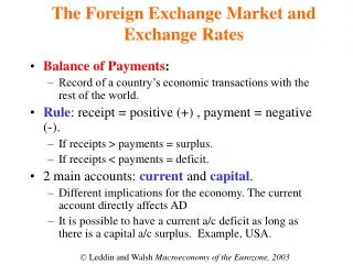
Current account and capital account • The current account is not the only element of international trade. • The balance of payments composed of: • The current account CA: • Tracks outflows minus inflows of goods and services • It corresponds to the Exports – Imports component. • The capital account KA: • Tracks inflows minus outflows of capital of a country • Either as direct investment (building factories, etc) • Or purchases/sales of assets

Current account and capital account • The current account was explained in the previous section as the ‘net exports’ added to C + I + G. • What role does the capital account play ? • To understand their relation, let’s derive the savings/investment balance for an open economy • Setting Z = Y :

Current account and capital account • This gives us the equilibrium condition in terms of investment and savings: • Simplifying assumption: the government budget is in equilibrium (G-T = 0) • If there is a CA deficit (X-M < 0), there are not enough savings (agents are spending too much). Some of the financing of investment (I) must come from abroad. • If there is a CA surplus (X-M > 0), there is excess savings (agents are not spending enough). The excess saving are used to fund foreign investment. • The adjustment to the current account balance occurs through an inflow or outflow of savings: This is the capital account.

Current account and capital account • The BoP is in equilibrium when • CA+KA = 0 • The current account and capital imbalances add to 0 • As seen in the previous slide, this is equivalent to saying that S = I in an open economy

Current account and capital account Source: BIS,2007 World Report

Current account and capital account • The USA have been net importers and net borrowers since the 1980’s. The US current account deficit in 2006 was 6,6% of its GDP. • Europe has recently seen positive balances on its current account, which reflects a relatively low level of growth. • Japan has traditionally been a net exporter and a net lender. • The current accounts surpluses of emerging Asian countries (particularly China) have grown during the 1990’s

Current account and capital account • The amount of savings required to finance the current account deficit of the USA has tripled since 1997. • On the other had, the emerging economies have become net providers of savings flows. • Europe and Asia (including Japan) has covered 2/3 of the funding needs of the USA in 2002.

From IS-LM to Mundell-Fleming • Model developed by Robert Mundell and Marcus Fleming • It extends the IS-LM model to an open economy • Aggregate demand now contains the current account : i.e. the difference between exports and imports. • X(Y*,e) : Exports are a function of the income of the rest of the world (exogenous) and the exchange rate • M(Y,e) : Imports are a function of national income and the exchange rate

From IS-LM to Mundell-Fleming Determinants of the current account: • If e increases (depreciation): exports are more competitive and imports more expensive. The net balance of the current account increases. • If Y increases: imports increase and the net balance of the current account falls. • Y* is exogenous, and Y is already determined in IS-LM. There is an extra variable to account for: the exchange rate e. • We need to add another equation (market) in order to be able to solve the system: we use the equilibrium condition on the balance of payments

From IS-LM to Mundell-Fleming • Reminder: the balance of payments is the sum of the current account and the capital account: • The equilibrium exchange rate is achieved when BP is equal to zero, in other words when the deficits and surpluses of the two accounts compensate exactly. • One can see that this equilibrium condition can be expressed in the (Y,i) space of IS-LM. • We still need to relate the exchange rate e to these variables

From IS-LM to Mundell-Fleming • The capital account (KA) • Is in surplus if the inflows of capital are larger than the outflows. • Is in deficit in the other case. • What determines these capital flows ? • Intuitive answer: the earnings on savings • If savings earn a higher return in Europe compared to the USA, one would expect American capital to flow towards Europe.

From IS-LM to Mundell-Fleming • Investors choose between assets that pay different interest rates in different currencies. • What is the expected return for each of the possible investment? • Their decision needs to account for the interest rate differentials… • …But also for the evolution of the exchange rates between currencies. • This arbitrage mechanism produces what is called the uncovered interest rate parity (UIRP) • This gives us a relation between interest rate differentials and changes in the exchange rate

From IS-LM to Mundell-Fleming • You are a European investor with capital K (in €) looking for a 1-year investment. • You can invest in €-denominated bonds, and after a year you earn: • Or you can buy $-denominated US bonds: • Step 1: you first convert your capital into dollars: • Step 2: after a year, you’ve earned (in dollars):

From IS-LM to Mundell-Fleming • But you need to bring you investment back home ! • In other words you need to convert your capital in $ back into €. • In the mean time the $/€ exchange rate may have changed • Step 3: you convert your investment into € • You are indifferent if the 2 returns are equal

From IS-LM to Mundell-Fleming • You’re indifferent between $ and € assets if: • Rearranging gives: • If the exchange rate is not too volatile, this can be expressed as:

Expected exchange rate depreciation Home interest rate World interest rate From IS-LM to Mundell-Fleming • Let’s summarise: Capital flows ensure an equalisation of interest rates expressed in the same currency • If the home interest rate is higher than world interest rate, zero net capital flows between countries requires investors to be expecting a depreciation of the home currency. • If this is not the case, then capital will flow into the home country, appreciating e until depreciation expectations occur • Only if the home rate equals the foreign rate will depreciation/appreciation expectations be zero (equilibrium)

From IS-LM to Mundell-Fleming • On BP the balance of payments is in equilibrium i BoP surplus Appreciation of e • BP is upward-sloping • An increase in Y leads to a BoP deficit (CA deficit) • Returning to equilibrium requires a KA surplus, and hence a higher i BP KA surplus • The slope depends on the internationa mobility of capital • The lower capital mobility, the larger the slope of BP. CA deficit BoP deficit Depreciation of e Y

BP From IS-LM to Mundell-Fleming • The MF model was developped in the 60’s, when capital mobility was low (Bretton Woods) Perfect capital mobility i=i* i BoP Surplus Appreciation of e • As a simplification, nowadays we assume perfect capital mobility i* • However, this remains a simplification! • For certain cases (like the case of trade with China), The concept of imperfect capital mobility remains relevant. BoP Deficit Depreciation of e Y

From IS-LM to Mundell-Fleming • We now have 3 curves, IS-LM-BP : i LM BP i* IS Y

The effectiveness of policy • We now move to assessing the effectiveness of policy under the possible exchange rate settings:

The effectiveness of policy • Monetary policy with fixed exchange rate: i • LM shifts to the right • The increase in the money supply lowers the rate of interest, leading to depreciation pressures on e LM BP • In order to guarantee the fixed exchange rate the CB must immediately increase i to i=i* by reducing money supply i* IS • Such a policy cannot be carried out in practice Y

The effectiveness of policy • Fiscal policy with fixed exchange rate: i • IS shifts to the right: • The crowding out effect increases the rate of interest, creating appreciation pressures on e LM BP • In order to guarantee the fixed exchange rate the CB must immediately reduce i to i=i* by increasing money supply i* IS • Policy is effective in increasing Y Y

The effectiveness of policy • Monetary policy with flexible exchange rate: i • LM shifts to the right • The interest rate falls, which leads to a depreciation of the exchange rate e LM • The depreciation of the exchange rate stimulates exports and penalises imports • As a resut IS shifts to the right BP i* IS • Policy is effective Y

The effectiveness of policy • Fiscal policy with flexible exchange rate: i • IS shifts to the right • The Central Bank doesn’t have to react: The interest rate increases and the exchange rate appreciates LM BP • The appreciation of the exchange rate penalises exports and stimulates imports • IS shifts left i* IS • Policy is ineffective Y

The effectiveness of policy • Summarising all this: • Even with this simple example (assumption of perfect capital mobility), one can see that the effectiveness of policy depends on international conditions!

The effectiveness of policy Monetary Union Incompatibility Triangle (Mundell) Capital mobility Fixed exchange rate Flexible Exchange rate Financial Autarky Autonomous monetary policy

Exchange rates and the Mundell-Fleming model