Forecasting convective outbreaks using thermodynamic diagrams.

1. Forecasting convective outbreaks using thermodynamic diagrams. Anthony R. Lupo Atms 4310 / 7310 Lab 10

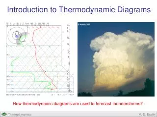
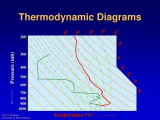
2. Forecasting convective outbreaks using thermodynamic diagrams. • *Recall early in the semester we talked about determining the LCL, CCL, LFC, and EL using a thermodynamic diagram. • We also talked about calculating the LI and the SI. These indicies based on the principle that warmer air parcels (parcels warmer that the environment will rise under their own power).

3. Forecasting convective outbreaks using thermodynamic diagrams. • The warmer the air parcels are over the environment the stronger the bouyant force. This indicates greater atmospheric instability and is correlated with severe weather outbreaks. • If parcels are cooler than the environment, the cooler parcels fall back to their original place. • Convective Available Potential Energy (CAPE)

4. Forecasting convective outbreaks using thermodynamic diagrams. • Convective Available Potential Energy (CAPE) • CAPE  Positive (+ ) - then parcels warmer than their environment. The environment gains energy from the air parcels. •  Negative (-) parcels cooler than their environment. Environment must do work to lift parcels and loses energy.

5. Forecasting convective outbreaks using thermodynamic diagrams. • The bouyant force can be defined as: • where g is gravity (the restoring force) • and Tv’ is the parcel virtual temperature.

6. Forecasting convective outbreaks using thermodynamic diagrams. • Thus it should be apparent that: •  if you are cooler than the environmental temperature, then B is negative •  if you are warmer than the environmental temperature, then B is positive.

7. Forecasting convective outbreaks using thermodynamic diagrams. • If we integrate from LFC to EL (invoke il serpente): • CAPE is given in units of Joules. (Or Joules per unit mass).

8. Forecasting convective outbreaks using thermodynamic diagrams. • CAPE is rapidly becoming the index of choice for severe weather forecasters (Pass out Rochette et al. 2000) • Many different empirical CAPE quantities – such as BEST CAPE, or MU CAPE – calculate by starting with the parcel with the highest qe

9. Forecasting convective outbreaks using thermodynamic diagrams. • Now let’s take a look at the dynamical effect of B and relate to vertical motion (ignore x,y): • Invoke “uzh”

10. Forecasting convective outbreaks using thermodynamic diagrams. • Typical values of CAPE that lead to severe weather. Of course these can be different for different locales, and different types of CAPE (what color is your CAPE?), but in general: • Values of CAPE: •  Moderate to strong convection occurs with CAPE values of 1000 – 3000 J/kg •  Very strong convective outbreaks 3000 – 5000 J/ kg •  Max observed CAPEs. 5000 – 7000 J/kg

11. Forecasting convective outbreaks using thermodynamic diagrams. • For CAPE of 2500 J/kg: • wmax = square root of 2 CAPE or approximately 70 m/s • The computation of CAPE is sensitive to location of LCL and LFC which means that this is sensitive to moisture and dew points (mixing ratios) in the lowest 500 m of the PBL.

12. Forecasting convective outbreaks using thermodynamic diagrams. • If there is a “capping inversion” or stable layer above a moist unstable boundary layer, This is Convective Inhibition (CIN) In this Case: B is (-). • Then the integral from LCL to LFC is CIN, it’s the measure of the strength of the capping inversion. From that we can calculate the strength of the forced vertical motion necessary to “bust the cap”.

13. Forecasting convective outbreaks using thermodynamic diagrams. • The measurement of convective inhibition:

14. Forecasting convective outbreaks using thermodynamic diagrams. • Thus for a CIN of 200 J/kg a forced rise of 20 m/s is needed to “bust the cap”. • Typical severe weather soundings (Bluestein Vol II p 445 – 455) • The Air Force (Col. Miller, 1940’s through 1970’s) did much severe weather research including the compilation of many soundings and their characteristics w/r/t severe weather (hail, wind gust etc.)

15. Forecasting convective outbreaks using thermodynamic diagrams. • Miller Type 1 “loaded gun” sounding •  Moist well mixed (q, and RH) PBL separated from a very dry layer above by a stable layer. •  Lapse rate is nearly dry adiabatic Above “cap” stable layer. •  Depth of the mosit layer typically 1500 m (150 hPa), and sfc dewpoints typically 10 C or better near sfc and 8 C or better at top of PBL (well-mixed!!)

16. Forecasting convective outbreaks using thermodynamic diagrams. • Sounding

17. Forecasting convective outbreaks using thermodynamic diagrams. • High qe laspe rates and CAPEs high, and SI and LI low. •  Common for plains region, potential for very strong intense updrafts. Strong cool downdrafts likely. • Miller Type II •  Common in tropics and more common to severe weather east of Mississippi river.

18. Forecasting convective outbreaks using thermodynamic diagrams. •  Deep layer of moisture up to 7 km. (RH > 65%) •  Sounding either moist adiabtic or conditionally unstable. Lower CAPEs •  No capping inversion. • Miller Type III •  Similar to type II (no cap and moist adiabatic or conditionally unstable)

19. Forecasting convective outbreaks using thermodynamic diagrams. • Sounding (big outbreak 2011)

20. Forecasting convective outbreaks using thermodynamic diagrams. •  but temps 10 – 15 C cooler, and the moist layer is more shallow •  Cold air sounding, more typical of cold lows near cold core closed Ls or troughs. Thus convection is not widespread. (LOWER CAPEs) • Miller Type IV • Common in high plains and desert in summer. • Warm dry CT airmass, under cool maritime polar airmass.

21. Forecasting convective outbreaks using thermodynamic diagrams. • Sounding

22. Forecasting convective outbreaks using thermodynamic diagrams. • Sounding type 4

23. Forecasting convective outbreaks using thermodynamic diagrams. •  PBL dry adiabatic, layer above moist adiabatic. • Very high based convection,frequently no rain but lightning and strong downdrafts. • Lifted Index • Showalter Index • Energy Index:

24. Forecasting convective outbreaks using thermodynamic diagrams. • The End!

25. Forecasting convective outbreaks using thermodynamic diagrams. • Questions? • Comments? • Criticisms? • LupoA@missouri.edu

26. Forecasting convective outbreaks using thermodynamic diagrams.