Download
1 / 35
350 likes | 586 Views
Modelling of non-equilibrium turbulent flows. Tania S. Klein Second Year PhD Student. Supervisors: Prof. Iacovides and Dr. Craft. School of MACE, The University of Manchester. Outline of Presentation. Introduction Test Cases Turbulence Models Results Conclusions.

E N D
Modelling of non-equilibrium turbulent flows Tania S. Klein Second Year PhD Student Supervisors: Prof. Iacovides and Dr. Craft School of MACE, The University of Manchester
Outline of Presentation • Introduction • Test Cases • Turbulence Models • Results • Conclusions
Introduction Non-equilibrium flows: those subjected to rapid changes Sudden contraction, sudden expansion Imposed pressure gradients They are commonly found in the industry: Valves, pumps, heat exchangers, curve surfaces Objective of this work: Test different turbulence models for several cases in order to evaluate their performance.
Test Cases • Fully Developed Channel Flow • Homogeneous Constant Shear Flow • Zero Pressure Gradient Boundary Layer • Adverse Pressure Gradient Boundary Layer • Favourable Pressure Gradient Boundary Layer • Contraction/Expansion Flows
Fully Developed Channel Flow • One of the simplest flows: • 2D • DP=cte • U=U(y) Simulated Cases ERCOFTAC database Kawamura Lab
Homogeneous Constant Shear Flow S=dU/dy=cte U = U(y) not wall-bounded unsteady
Zero Pressure Gradient Boundary Layer Simulated Cases • Still a simple flow: • 2D • DP=0 • U=U(x,y)
Adverse Pressure Gradient Boundary Layer • Non-equilibrium flow: • 2D • DP > 0 • U=U(x,y) • dU/dx < 0 S&J M&P
Favourable Pressure Gradient Boundary Layer • Non-equilibrium flow: • 2D • DP < 0 • U=U(x,y) • dU/dx > 0 • reaches a self-similar prolife
Contraction/Expansion Flows • Non-equilibrium flow: • 3D • dV/dy = cte • dW/dz = -cte a= 0 a= /2
Turbulence Models *Run with the wall function of Chieng and Launder (1980)
Results Fully Developed Channel Flow General Conclusions • All models predicted the log law reasonably well. • All models predicted the shear Reynolds Stress reasonably well. • The HJ and TC models best predicted the normal Reynolds stresses.
Results Fully Developed Channel Flow Re = 6500
Results Fully Developed Channel Flow Re = 6500
Results Fully Developed Channel Flow Re = 41441
Results Homogeneous Constant Shear Flow General Conclusions • Difficult prediction • Overall, the SG and the KS model performed best • The extreme shear values are more difficult to predict. S=20√2 ; S0+=1.68 S=10 ; S0+=16.76
Results Homogeneous Constant Shear Flow S=20√2 S0+=1.68
Results Homogeneous Constant Shear Flow S=20√2 S0+=30.75
Results Zero Pressure Gradient BL General Conclusions • The tested turbulence models have shown to be sensitive to the inlet conditions, implying bad predictions at low Req values. • The normal Reynolds stresses were better predicted by the RST models, as expected. • One can notice the importance of LRN models for the near wall region predictions.
Results Zero Pressure Gradient BL
Results Zero Pressure Gradient BL
Results Adverse Pressure Gradient BL • The BL parameters (Cf, d, d*, q and H) were reasonably well predicted by all turbulence models. • The U and uv profiles were captured by all turbulence models up to station T5 in the S&J case. The same has not occurred for the M&P cases. • The RST models best predicted the normal Reynolds stresses, however the best model varies from case to case; station to station… General Conclusions
Results Adverse Pressure Gradient BL S&J
Results Adverse Pressure Gradient BL M&P
Results Adverse Pressure Gradient BL M&P
Results Favourable Pressure Gradient BL General Conclusions • The turbulence model which overall better predicted these flows was the KS model, although it failed to predict the Reynolds stresses. • The KS and LS models are the only ones expected to correctly predict the laminarization process, since they possess a term which accounts for the second derivative of the mean velocities. • The RST models best predicted the normal Reynolds stresses, specially the TC and HJ models.
Results Favourable Pressure Gradient BL K=1.5x10⁻⁶
Results Favourable Pressure Gradient BL K=1.5x10⁻⁶
Results Favourable Pressure Gradient BL K=2.5x10⁻⁶
Results Favourable Pressure Gradient BL K=2.5x10⁻⁶
Results Contraction/Expansion Flows General Conclusions • No turbulence model was able to correctly predict the interruption of the applied strains. • Overall, the GL and the TC models provided the best predictions. • The eddy viscosity formulations clearly failed to predict these flows.
Results Contraction/Expansion Flows T&R
Results Contraction/Expansion Flows G&M - a = /2
Conclusions • The Channel flow, which is the simplest flow, was reasonably well predicted by all turbulence models as well as the ZPGBL cases at high Req values. • The two not wall-bounded cases – HCS flow and C/E flows – were the most difficult to predict and the RST models performed better, showing the importance of calculating the Reynolds stresses through transport equations. • The APGBL cases could not be well predicted by any model at high DP, however the FM model could match the U profile. • The FPGBL cases were better predicted by the KS model which evidenced the importance of a velocity second derivative term to predict laminarization.