Download
1 / 16
240 likes | 1.01k Views
Correlation. Simple correlation between two variables Multiple and Partial correlations between one variable and a set of other variables Canonical Correlation between two sets of variables each containing more than one variable.

E N D
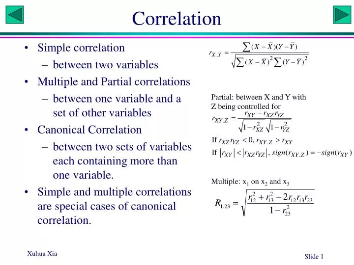
Correlation • Simple correlation • between two variables • Multiple and Partial correlations • between one variable and a set of other variables • Canonical Correlation • between two sets of variables each containing more than one variable. • Simple and multiple correlations are special cases of canonical correlation. Partial: between X and Y with Z being controlled for Multiple: x1 on x2 and x3
Review of correlation X Z Y 1 4 14.0000 1 5 17.9087 1 6 16.3255 2 3 14.4441 2 4 15.2952 2 5 19.1587 2 6 16.0299 2 5 17.0000 3 3 14.7556 3 4 17.6823 3 5 20.5301 3 6 21.6408 4 3 15.0903 4 4 18.1603 4 5 22.2471 5 2 14.4450 5 3 16.5554 5 4 21.0047 5 5 22.0000 6 1 19.0000 6 2 18.0000 6 3 18.1863 6 4 21.0000 Compute Pearson correlation coefficients between X and Z, X and Y and Z and Y. Compute partial correlation coefficient between X and Y, controlling for Z (i.e., the correlation coefficient between X and Y when Z is held constant), by using the equation in the previous slide. Run SAS to verify your calculation: proc corr pearson; var X Y; partial Z; run;
Many Possible Correlations • With multiple DV’s and IV’s, there could be many correlation patterns: • Variable A in the DV set could be correlated to variables a, b, c in the IV set • Variable B in the DV set could be correlated to variables c, d in the IV set • Variable C in the DV set could be correlated to variables a, c, e in the IV set • With these plethora of possible correlated relationships, what is the best way of summarizing them?
Dealing with Two Sets of Variables • The simple correlation approach: • For N DV’s and M IV’s, calculate the simple correlation coefficient between each of N DV’s and each of M IV’s, yielding a total of N*M correlation coefficients • The multiple correlation approach: • For N DV’s and M IV’s, calculate multiple or partial correlation coefficients between each of N DV’s and the set of M IV’s, yielding a total of N correlation coefficients • The canonical correlation • Note: All these deal with linear correlations
Fitness Data /* First three variables: physical Last three variables: exercise Middle-aged men */ data fit; input weight waist pulse chins situps jumps @@; cards; 191 36 50 5 162 60 189 37 52 2 130 60 193 38 58 12 101 101 162 35 62 12 145 37 189 35 46 13 145 58 182 36 56 4 141 42 211 38 56 8 151 38 167 34 60 6 155 40 176 31 74 15 200 40 154 30 56 17 251 250 169 34 50 17 120 38 166 33 52 13 210 115 154 34 64 14 215 105 247 46 50 1 50 50 193 36 46 6 170 31 202 37 62 12 120 120 176 37 54 4 160 25 157 32 52 11 230 80 156 33 54 15 215 73 138 33 68 2 150 43 ;
SAS Program proc cancorr data=fit vdep wdep smc stb t probt vprefix=PHYS vname='Physical Measurements' wprefix=EXER wname='Exercises'; var weight waist pulse; with chins situps jumps; title2 'Middle-aged Men in a Health Fitness Club'; title3 'Data Courtesy of Dr. A. C. Linnerud, NC State Univ.'; run; What’s the meaning of these cryptic terms?Next slide
SAS Program • SHORT - suppresses all default output except the tables of Canonical correlations and multivariate statistics. • VDEP - requests multiple regression analyses with the VAR variable as dependent variables and the WITH variables as regressors. WDEP does the opposite • SMC - prints squared multiple correlations and F tests for the regression analyses • The STB option requests standardized regression coefficients. • VPREFIX - specify a variable prefix for canonical variables instead of using the default V1, V2, and so on. WPREFIX does the same. proc cancorr data=fit short vdep wdep smc stb t probt
Multiple Correlations DV: the Physical Measurements IV: Exercises Squared Multiple Correlations and F Tests 3 numerator df 16 denominator df 95% CI for R2 R2 R2.adj Lower Upper F Pr > F weight 0.517798 0.427385 0.065 0.736 5.73 0.0074 waist 0.752679 0.706306 0.380 0.877 16.23 <.0001 pulse 0.037362 -.143132 0.000 0.177 0.21 0.8901 Weight and WAIST are significantly associated with the exercise variables.
Regression of Phys. on Exer. Standardized Regression Coefficients weight waist pulse chins -0.1059 -0.2791 0.1281 situps -0.7273 -0.7640 0.1351 jumps 0.1619 0.1465 -0.0909 t Values for the Regression Coefficients weight waist pulse chins -0.4957 -1.8243 0.4244 situps -3.4776 -5.1007 0.4571 jumps 0.7768 0.9809 -0.3087 Prob > |t| for the Regression Coefficients weight waist pulse chins 0.6268 0.0868 0.6769 situps 0.0031 0.0001 0.6537 jumps 0.4486 0.3412 0.7615
Multiple Correlations DV: Exercises IV: the Physical Measurements Squared Multiple Correlations and F Tests 3 numerator df 16 denominator df 95% CI for R2 R2 R2.adj Lower Upper F Pr> F chins 0.408377 0.297448 0.000 0.657 3.68 0.0344 situps 0.716127 0.662901 0.316 0.857 13.45 0.0001 jumps 0.144544 -.015853 0.000 0.395 0.90 0.4622
Regression of Exer. on Phys. Standardized Regression Coefficients chins situps jumps weight 0.4994 0.0468 0.2802 waist -1.0261 -0.9209 -0.6102 pulse -0.0085 -0.1324 -0.0658 t Values for the Regression Coefficients chins situps jumps weight 1.2653 0.1710 0.5904 waist -2.6335 -3.4120 -1.3024 pulse -0.0411 -0.9249 -0.2649 Prob > |t| for the Regression Coefficients chins situps jumps weight 0.2239 0.8664 0.5632 waist 0.0181 0.0036 0.2112 pulse 0.9678 0.3688 0.7945
Canonical Correlation • Adjusted Approx Squared • Canonical Canonical Standard Canonical • Correlation Correlation Error Correlation • 1 0.878578 0.856195 0.052330 0.771899 • 2 0.264992 0.080853 0.213306 0.070221 • 3 0.062661 . 0.228515 0.003926 • Eigenvalue Difference Proportion Cumulative • 1 3.3840 3.3085 0.9771 0.9771 • 2 0.0755 0.0716 0.0218 0.9989 • 0.0039 0.0011 1.0000 • Significance test: • Eigenvalue Likelihood Approximate • Ratio F Value Num DF Den DF Pr > F • 1 0.21125051 3.40 9 34.223 0.0044 • 2 0.92612863 0.29 4 30 0.8799 • 3 0.99607358 0.06 1 16 0.8049
Standardized Canonical Coefficients for the Physical Measurements PHYS1 PHYS2 PHYS3 weight -0.1899 2.0261 0.2691 waist 1.1929 -1.5800 -0.4314 pulse 0.1218 0.3245 -1.0176 for the exercises EXER1 EXER2 EXER3 chins -0.3383 1.0114 -0.6139 situps -0.8614 -0.8403 -0.0579 jumps 0.1512 0.2536 1.1640 Because the variables are not measured in the same units, the standardized coefficients rather than the raw coefficients should be interpreted.
Canonical Structure: correlations Between Phys. and their canonical var.: PHYS1 PHYS2 PHYS3 weight 0.8028 0.5335 0.2662 waist 0.9872 0.0737 0.1416 pulse -0.2061 0.1098 -0.9723 Between Exer. and their canonical var.: EXER1 EXER2 EXER3 chins -0.6945 0.7165 -0.0658 situps -0.9609 -0.2169 0.1721 jumps -0.4141 0.3671 0.8329 Between Phys. and the canonical var. of Exer.: EXER1 EXER2 EXER3 weight 0.7054 0.1414 0.0167 waist 0.8673 0.0195 0.0089 pulse -0.1811 0.0291 -0.0609 Between Exer. and the canonical var. of Phys.: PHYS1 PHYS2 PHYS3 chins -0.6102 0.1899 -0.0041 situps -0.8442 -0.0575 0.0108 jumps -0.3638 0.0973 0.0522
Ecology data data candata; input Sp1 Sp2 Sp3 Sp4 Chem1 Chem2 Chem3 Chem4; cards; 21.09 21.90 9.19 9.18 20.96 21.52 7.46 7.41 14.69 14.85 14.06 14.07 14.80 14.63 13.71 13.69 2.11 2.17 3.13 3.06 3.17 2.43 2.10 1.96 9.58 9.47 8.14 8.06 9.54 9.71 9.36 9.43 10.02 10.71 9.02 9.06 11.16 10.59 10.91 11.10 14.65 14.32 15.10 15.15 14.59 14.61 13.55 13.55 24.42 24.12 6.00 6.12 24.36 24.50 4.30 4.34 22.20 22.10 4.14 4.04 23.37 22.74 4.90 5.06 8.34 8.88 9.16 9.06 8.75 8.19 7.59 7.58 10.49 10.12 11.08 11.13 10.09 10.73 9.55 9.56 25.72 25.91 1.12 1.16 25.94 26.01 1.98 1.99 4.16 4.44 3.05 3.09 3.97 4.89 4.53 4.53 12.07 12.31 11.09 11.15 12.68 12.89 12.62 12.78 19.13 19.36 11.13 11.05 18.69 19.05 9.01 9.16 5.80 5.15 4.11 4.18 6.07 6.33 5.10 4.96 1.27 1.15 2.10 2.17 1.27 1.80 0.73 0.75 22.15 22.52 8.01 8.04 22.08 22.53 7.43 7.31 26.53 26.27 0.14 0.11 26.33 26.88 0.55 0.57 17.25 17.68 11.12 11.18 17.39 17.76 9.51 9.55 7.94 7.46 6.13 6.03 7.53 7.67 7.51 7.47 4.12 4.45 3.08 3.14 5.21 4.65 3.92 4.00 17.59 17.53 11.19 11.04 16.97 16.70 12.30 12.26 15.41 15.16 13.12 13.03 15.79 16.01 12.00 11.83 12.90 12.93 11.12 11.12 12.80 12.04 11.52 11.52 19.14 19.11 7.16 7.14 19.88 19.84 8.86 8.90 25.11 25.50 3.13 3.20 25.28 25.44 4.26 4.23 ;
SAS Program (cont.) proc cancorr vdep wdep smc stb t probt vprefix=BIO vname='Species' wprefix=ENV wname='Environment'; var Sp1 Sp2 Sp3 Sp4; with Chem1 Chem2 Chem3 Chem4; run; Run and explain