Download
1 / 25
270 likes | 581 Views
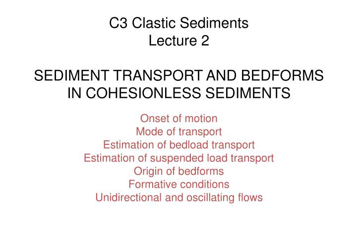
C3 Clastic Sediments Lecture 2 SEDIMENT TRANSPORT AND BEDFORMS IN COHESIONLESS SEDIMENTS Onset of motion Mode of transport Estimation of bedload transport Estimation of suspended load transport Origin of bedforms Formative conditions Unidirectional and oscillating flows.

E N D
C3 Clastic Sediments Lecture 2 SEDIMENT TRANSPORT AND BEDFORMS IN COHESIONLESS SEDIMENTS Onset of motion Mode of transport Estimation of bedload transport Estimation of suspended load transport Origin of bedforms Formative conditions Unidirectional and oscillating flows
DIMENSIONAL ANALYSIS OF MOTION THRESHOLD Variables: Critical bed shear stress, tc [ML-1T-2] repeat Fluid density, rf [ML-3] repeat Fluid viscosity, m [ML-1T-1] Grain diameter, D [L] repeat Submerged specific weight of grain, g ‘ [ML-2T-2] Sought: balance of inertial and viscous forces (Reynolds number), balance of gravitational and fluid forces. Combine g’ with repeating variables gives: t0/g‘D = (Shields’ Number). Combine m with repeating variables: (D√rf√t0)/m = (rfu*D)/m = u*D/n = Re* , where n = m/r is the kinematic viscosity. Remember: shear velocity u*2 = t0/r . Re* is boundary or bed Reynolds number. and Re* fully characterise onset of sediment motion. Their relation was constrained experimentally by Shields in 1936.
SHIELDS’ DIAGRAM Re* < 10: fine grain sizes: well-packed, cohesive sediment, enclosed within viscous sublayer. Entrainment more difficult than fine sand. Shields’ stress b increases with decreasing Re* Re* > 10: Non-cohesive silt and sand. Entrainment more difficult with increasing grainsize. Expected: Shields’ stress b increases with increasing Re* Experimental results: flat trend. Shear stress and grain size on both axes.
YALIN’S DIAGRAM b In Shields’ diagram: shear stress and grain size are on both axes in θ and Re*. Solve by combining bed Reynolds number with Shields’ θ to eliminate shear stress: = Re*2/ θ . Yalin’s plot of θ against √ has same general form as Shields’ curve, but has just material variables on the x-axis.
MOTION THRESHOLD Two special cases: Wind and glue Under WIND the first grains to move dislodge further grains (there is little viscous damping ) causing a chain reaction. The grains stay moving when U* is decreased to 80% of the “fluid threshold.” Bacteria grow on sand grains, producing a mucopolysaccharide “glue.” This can almost double the critical U*.
MODES OF SEDIMENT TRANSPORT BED LOAD Sliding, rolling, saltation SUSPENDED LOAD Mode of transport depends on grain density grain size flow hydraulics Conditions vary in space and time: Modes of transport change frequently. Distinction between bed load and suspended load is not easy. Transport stage
TRANSPORT STAGE u*/ws , where u* is the shear velocity, t0/r ws is the settling velocity (cf. Stoke’s law). With increasing shear velocity, proportion of load moving in suspension increases. Therefore dimensionless grain velocity ug/U increases with transport stage. Here, ug is the grain velocity, and U is the flow velocity. u* = ws approximates saltation – suspension threshold. When u* > ws, then grains move with approximately the velocity of the flow. Results shown for quartz sand in flow 48 mm deep.
BEDLOAD TRANSPORT • Bedload transport rate Qb ~ stream power, w = t0u . • conversion factor to be constrained empirically • Prediction of bedload transport complicated by: • bed armouring and consolidation of gravels. • resistance of bedforms in sand and gravel rivers. • (some of the bed shear stress moves seds, some is ‘form drag’) • unsteadiness in high stage flows. • has dimensions [ML2T-3] over unit area of stream bed [L2]: • Qb isproportional to the cube of (excess) flow velocity. • Qb (U-Uc)3 (u*- u*c)3
SUSPENDED LOAD Observed suspended sediment concentration profiles are not linear in depth C incr to the bed. Key is settling velocity of grains. Concentration profile reflects balance of upward diffusion and gravitational settling of grains. When C is constant in time, then any loss of sediment due to settling is balanced by upward diffusion of sediment. Settling flux is wC. Upward diffusion flux Q = -k dC/dy. wC = -k dC/dy , or dC/C = -wdy/kt , where kt = be, and e is the kinematic eddy viscosity. b ≈ 1, and e = u*[(h-y)/h]ky . Von Karman’s k = 0.4 . dC/C = whdy/[bku*(h-y)y] . Mississippi River at St. Louis
SUSPENDED LOAD dC/C = wshdy/[bku*(h-y)y] At reference height a, C = Ca . Integrate: C/Ca = [h-y/y × a/h-a]ws/bku*. This gives suspended sediment concentration at any depth in flow in relation to concentration at reference depth. Only need to know a and Ca. The grouping ws/bku* is the Rouse number. Since b ≈ 1, and k = 0.4, at a Rouse number of 2.5 ws = u*. This is a good criterion for suspension. If Rouse number > 2.5: ws > u*with bedload transport dominant. Suspended sediment transport rate is product of the mass of suspended sediment ms in a column of water over a unit area of bed and the depth-averaged flow velocity U at the station: Qs = msU
BEDFORMS UNDER SHEAR FLOW Antidunes grains stuck down Flat bed On flat bed, resistance to flow is due to boundary roughness: skin friction (~ grain size) Developing bedforms become main roughness element: form drag With increasing flow velocity : 1) bedforms grow, shear stress up. 2) dunes wash out, replaced by flat bed: shear stress down. 3) standing waves and antidunes form: shear stress up. Shear stress bad indicator of state of bed; use flow velocity.
FLOW REGIMES Upper flow regime Lower flow regime Cross-section of flow from a tap into a flat sink Hydraulic jump Froude number is dimensionless product expressing balance of inertial and gravitational forces Fr < 1: subcritical flow Fr > 1: supercritical flow
RIPPLE INITIATION ~100 dv Bedform wavelength Ripples form when random points of high boundary shear stress (sweeps) cause formation of a pile of grains. Pile of height dvcauses flow disturbance ~100 dvlong downstream, similar to the separation zone behind a ripple. D > 0.7 mm: grains disrupt viscous sublayer and discrete flow disturbances no longer occur. Ripples do not form, bed is plane.
FLOW OVER BEDFORM, MIGRATION & SEDIMENT FLUX Ripples and dunes formed under uni- directional flow have shallow upstream or stoss faces, dominated by rolling grains, and steep downstream or lee slopes, dominated by grain avalanching. Downstream flux of sediment due to bedform migration: where UB is speed of bedform, H is height of bedform, F is porosity of bed material.
BEDFORM SCALES Is similar for ripples and dunes, but ripples scale on grainsize while dunes scale on flow depth (L – wavelength), • Dunes:L ~ 2ph • dune height = h/3 to h/6 • where h is flow depth, • Ripples: height < 4 cm • ~ ≤ 1000d • and d is grain size. • Typically L = 10-60 cm
SEDIMENT FALLOUT Angle of climb and preservation of stoss and lee side are determined by balance of downstream translation and vertical build up. Climbing ripples
BEDFORMS PLANFORM AND INTERNAL STRUCTURE Basic bedform: crescent Planar cross stratification Trough cross stratification
BEDFORM STABILITY FIELDS There is a problem of ambiguity. In this diagram the bed phases are plotted on θ-d axes. There is a big overlap in stability fields of Upper Plane bed with Ripples and Dunes. There is no such ambiguity with flow speed, here the bedforms change monotonically with Ū. So Ū is to be preferred.
CONTROLS ON BEDFORM: DIMENSIONAL ANALYSIS Assumptions: steady and uniform flow, equilibrium bedforms, mean grain size describes bed material. Variables: Grain size D [L] Density of grains rs [ML-3] exclude Density of fluid rf [ML-3] repeat Viscosity of fluid m [ML-1T-1] repeat Gravitational acceleration g [LT-2] repeat Flow depth h[L] Flow velocity U [LT-1] Dimensionless Products: Experimental set up: Water, quartz sand, variable temperature. constant in temp
BEDFORM STABILITY FIELDS Flow depth: 0.25 – 0.40 m Upper plane bed in fine grains: Due to high sediment concentration damping turbulence. Absence of ripples in course sand: Lack of viscous sublayer over hydraulically rough boundary.
BEDFORM STABILITY FIELDS; FLOW REGIMES Super critical Upper Sub critical Lower flow regime
BEDFORM STABILITY FIELDS Bedform stability can be represented in 3D plot of standardized flow velocity, flow depth and grain size. Sections through this cube can be viewed. h10
BEDFORMS UNDER OSCILATORY WAVES Controls on bedform: Flow velocity Sediment grain size Wave period Form Index: L/H
New wave ripple stability diagrams Shaded region is zone of observed linear waves h-T-H-Uo Stability for 2 m wavelength ripples Trochoidal wave ripples are stable under “normal” conditions and can have large wavelengths and heights if grain size is also large. This counters the arguments of Allen & Hoffman for extreme climate conditions in the Snowball aftermath Bedform stability diagram for linear oscillatory waves as function of grain diameter and bedform wavelength. Shaded areas are of ambiguity Lamb et al, Geology, 40, 827-830, 2012