Intertemporal exchange

1. Intertemporal exchange Intertemporal exchange – trading current consumption for future consumption; i.e. lending and borrowing. Consumption smoothing – spending is ‘smoother’ than income over time.

2. $ Borrowing Saving labor income consumption Age Intertemporal exchange

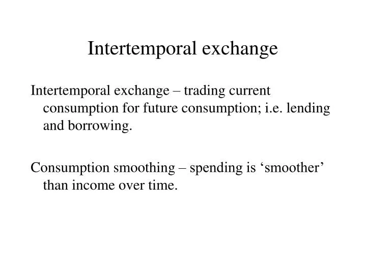
3. Intertemporal exchange • Households – net lenders • Firms, government – net borrowers Financial system exists to facilitate intertemporal exchange: borrowing and lending

4. Services of financial system • Reduce transactions costs of borrowing and lending • Allow risk-sharing • Provide liquidity • Providing information

5. Financial markets Direct finance – lenders and borrowers directly interact through the exchange of securities or financial instruments. Lenders buy securities of borrowers. • Primary and secondary markets • Debt and equity instruments/securities • Government debt • International borrowing and lending

6. Financial intermediaries Indirect finance – lenders lend to intermediaries, which in turn lend to borrowers; lenders do not directly hold securities of ultimate borrowers. Examples: banks (depository institutions), pension funds, insurance companies.

7. Asymmetric information Borrowers are better informed than lenders about the use of funds, leading to costs: • Adverse selection (the lemons problem) – costs associated with distinguishing good from bad borrowers. Before the transaction • Moral hazard – costs associated with verifying and monitoring borrower’s use of funds. After the transaction

8. Banks and asymmetric information • Specialize in obtaining relevant information. • Make private loans, so there are incentives for information gathering. • Require borrowers to put up collateral. Internal finance versus external finance.

9. US bank loans

10. Private loans versus securitization • Securitization of loans • An example: Fannie Mae, Freddie Mac and mortgage-backed securities Fannie and Freddie _____________________________________________ Mortgage loans $1,500 b | $1,350 b MBS | $ 150 b Equity

11. Fannie and Freddie MBS • Owners share cash flow (P&I) from underlying mortgages. • Different from bonds because of principal pre-payment. • Lower yields • Backed by pools of mortgages • Government guarantee of principal and interest (no longer implicit!)

12. Measuring interest rates • Interest rates in general measure the tradeoffs of intertemporal exchange – the marginal costs and benefits of current and future consumption. • Two concepts: • Yield-to-maturity = interest rate that equates the present value of a securities payoffs to its current price. • Rate of return = rate of gain or loss over a given holding period.

13. YTM: Multi-period coupon bond Any debt security is characterized by 1) price; 2) payoffs (face value and interest); and 3) timing of payoffs. P = price F = face (or maturity) value T = time to maturity x = coupon interest rate (not ytm) C = coupon interest payments (= xF) i = yield-to-maturity P = C/(1+i) + C/(1+i)² + … + C/(1+i)T + F/(1+i)T http://www.moneychimp.com/calculator/bond_yield_calculator.htm

14. Example 1 P = $975 F = $1000 T = 10 years x = 5% C = xF = $50 → i = .053329 = 5.329% Example 2 P = $1100 F = $1000 T = 10 years x = 5% C = xF = $50 → i = 3.781% YTM: Multi-period coupon bond

15. No coupon payment, but sells at a discount relative to face value. _____________ P = $900 F = $1000 T = 5 years x = 0% C = xF = 0 → i = 2.13% i = (F/P)(1/T) – 1 ______________ P = $900 F = $1000 T = 1 year x = 0% C = xF = 0 → i = 11.11% YTM: Discount bond

16. Rate of return R = rate of return P(t) = price of security at time t C(t) = payout during the period R = [P(t+1) + C(t+1) – P(t)]/P(t)

17. Rate of return: discount bond P = 900 F = 1000 T = 2 i = 5.41% P = 950 F = 1000 T = 1 i = 5.26% R = (950 – 900)/900 = 5.56 %

18. Rate of return: discount bond P = 900 F = 1000 T = 2 i = 5.41% P = 890 F = 1000 T = 1 i = 12.36% R = (890 – 900)/900 = –1.11 %

19. Return of return: stock Buy shares for $100, receive dividend of $5, sell for $110 after one year. R = 110 + 5 – 100 / 100 = 15%.

20. Amortized securities Principal and interest are repaid in fixed payments; principal is amortized over the term (e.g. mortgages). P = initial loan value (price) i = interest rate (yield to maturity) A = annual payments T = term to maturity P = A/(1+i) + A/(1+i)2 + … + A/(1+i)T A = [1/(1+i) + 1/(1+i)2 + … + 1/(1+i)T]-1 P

21. Pre-payment risk on mortgage F = $100,000 i = 8% (loan rate, which will equal yield to maturity only if loaned at par). Annual payment = [(1/1.08) + (1/1.08)2]-1 (100,000) = 56,077 Amortization table Year Payment Interest(.08*principal) P – I Principal 100,000 1 56,077 8,000 48,077 51,923 2 56,077 4,154 51,923 0 Purchase price: At par: 100,000 → i = 8% At premium: 102,811 = (56,077/1+i) + (56,077/(1+i)2) → i = 6% At discount: 97,324 → i = 10% Suppose the borrower pre-pays principal after one year. At par: 100,000 = (1/1+ytm) (56,077 + 51,923) → ytm = 8% At premium: 102,811 = (1/1+ytm) (56,077 + 51,923) → ytm = 5% (decreases from 6%) At discount: 97,324 = (1/1+ytm) (56,077 + 51,923) → ytm = 11% (increases from 10%)

22. Real versus nominal interest rates R = nominal rate (yield) r = real rate (yield) π = market’s expected rate of inflation → r = R – π The real interest rate is the return in terms of goods, not money. Real interest rates affect intertemporal choices, not nominal rates.

23. Indexed bonds Typical bonds are ‘nominal’: prices, payouts and interest rates are in terms of the nominal unit of account: $. Indexed bonds are in ‘real’ terms; interest and principal payments are adjusted for inflation.

24. Indexed bonds Example: US TIPS (since 1997) P = F = $1000 TIPS, T = 2 years, x = 5%. Actual inflation year 1 = 3% (not known at time of sale) Actual inflation year 2 = 4% (not known at time of sale) ------------------------ Interest payment in year 1 = (0.05)(1000)1.03 = $51.50 Interest payment in year 2 = (0.05)(1000)(1.03)1.04 = $53.56 Principal received at maturity = (1000)(1.03)1.04 = $1071.20 r = 5% (since purchased at face value) R (nominal yield) determined from: 1000 = 51.5/(1+R) + 53.05/(1+R)2 + 1060.9 /(1+R)2 ------------------------------------------ Inflation-indexed yield spread = R – r = π

25. Indexed bonds Example: Chile’s unidad de fomento (UF) • UF is an indexed unit of account: prices quoted in UF’s, although pesos are the media of exchange. • The value of the UF appreciates with the rate of consumer inflation in pesos. • In principle, same as using, say, gold to quote prices and pesos as medium of exchange. • Yields on deposits and securities quoted in UF are therefore indexed against Chilean peso inflation.

26. Indexed bonds Example: • Deposit UF100 in bank, which pays 5% interest. • Initial UF value is 1000 pesos; during the year, peso inflation is 10%, so UF will be worth 1100 pesos. • In one year, receive UF105, which is equivalent to 115,500 pesos (105*1100). • Thus, 5% is the real rate of interest.

30. The loanable funds model of interest rates • Goal: explain fluctuations in interest rates. • Method: develop model of market for borrowing and lending funds. • Lending comes from households who save. • Borrowing comes from firms and government to finance spending. • Real interest matters for lending and borrowing decisions.

31. The loanable funds model of interest rates Assumptions about economic behavior: Lenders – the quantity of lending (supply of loanable funds) is positively related to real market interest rates: the higher is the rate, the greater the opportunity cost to savers of current consumption. This relationship is reflected in the upward slope of the supply curve. Borrowers – the quantity of borrowing (demand for loanable funds) is negatively related to market interest rates: the higher the rate, the greater the opportunity cost to borrowers of current expenditures. This relationship is reflected in the downward slope of the demand curve.

32. The loanable funds model of interest rates Equilibrium – market interest rates adjust until the supply and demand for loanable funds are equal. In equilibrium, there is an efficient allocation of loanable funds. In the graphs to follow, we assume that π is ‘fixed’ (doesn’t adjust to changes in the market for loanable funds). So changes in R (nominal) reflect changes in r (real).

33. interest rate (R) Supply (saving, lending) r* Demand (spending, borrowing) Loanable funds The loanable funds model of interest rates

34. Explaining interest rate fluctuations Equilibrium interest rates will change in when the supply and demand curves for loanable funds shift. Factors (besides interest rates) that make lending/saving more desirable or feasible shift the supply curve to the right (and vice versa). Factors (besides interest rates) that increase the demand for borrowing shift the demand for loanable funds to the right (and vice versa).

35. Interest rate (R) Supply (saving, lending) r1 r* Demand (spending, borrowing) Loanable funds A decrease in the supply of loanable funds

36. Interest rate (R) Supply (saving, lending) r* Demand (spending, borrowing) Loanable funds An increase in the demand for loanable funds

37. Increases in the supply of loanable funds • Increase in household income • Decrease in wealth (holding income constant) • Decrease in current taxes (if households perceive that they must be followed by increases in future taxes) • Reduction in the risk of financial assets (lower default risk) • Increase in the liquidity of securities (e.g. introduction of secondary market). • A decrease in information costs of adverse selection and moral hazard. • A decrease in expected inflation.

38. Increases in the demand for loanable funds • Increase in the marginal product of capital • Increase in the government’s budget deficit • Increase in expected inflation (reduces the real rate for any given nominal rate) • Increase in the country’s trade surplus, or reduction in the country’s trade deficit (reflects borrowing by foreigners)

39. S_L Interest rate S_d R_L R_d D Loanable funds Financial intermediation

40. Interest rate (R) Supply (saving, lending) r* Demand (spending, borrowing) Loanable funds Increase in government deficit

41. Interest rate (R) Supply (saving, lending) R1 R0 Demand (spending, borrowing) Loanable funds Increase in expected inflation

42. Changes in the expected rate of inflation cause nominal rates one-for-one, without affecting the real rate. This hypothesis is likely valid in the long-run, not the short-run. Fisher Hypothesis Irving Fisher, 1867-1947

43. Yield spread

45. Term structure of interest rates • Relationship between interest rates of bonds identical except in term to maturity. • Yield curve: plot of yields (rates) as a function of maturity. For example, an upward sloped yield curve shows that longer-term yields are higher than shorter term yields.

47. The Expectations Hypothesis Example: 2-year planning horizon 1) buy a two-year discount bond (T=2) 2) buy a discount bond with T=1, then when that bond matures after one year, buy another one-year bond. r1 = yield on 1 year bond Er2 = expected yield on 1 year bond in year 2 i = yield on 2 year bond Expectations hypothesis: (1 + i)² = (1 + r1 )(1 + Er2 ) i = ½ (r1 + Er2)

48. % 5 4 2 Term The Expectations Hypothesis Do these work for the yield curve below? r1 = 2%, Er2 = 6%, Er3 = 7% 1 2 3

49. Exchange Rates Markets for foreign exchange arise to facilitate international trade in goods and assets. These markets determine the exchange rate – the price of one currency in terms of another. The exchange rate determines the price of goods and assets purchased and sold abroad.

50. Exchange Rates Example: Price of Big Mac in US is $3.41 Price of Big Mac in UK is £1.99 Dollar-Pound exchange rate is $2.01/ £ → $ price of a Big Mac in UK = 1.99x2.01 = $4.00 → £ price of a Big Mac in US = 3.41/2.01 = £ 1.70 Real Big Mac exchange rate = (4 / 3.41) = 1.17 US Big Macs for 1 UK Big Mac With £1.99 you could get one Big Mac in the UK or 1.17 Big Macs in the US.