Download
1 / 23
230 likes | 238 Views
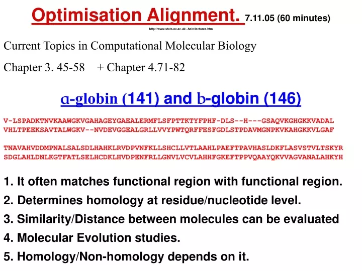
Optimisation Alignment. 7.11.05 (60 minutes) http://www.stats.ox.ac.uk/~hein/lectures.htm. Current Topics in Computational Molecular Biology Chapter 3. 45-58 + Chapter 4.71-82. a -globin ( 141) and b -globin (146) V-LSPADKTNVKAAWGKVGAHAGEYGAEALERMFLSFPTTKTYFPHF-DLS--H---GSAQVKGHGKKVADAL

E N D
Optimisation Alignment. 7.11.05 (60 minutes) http://www.stats.ox.ac.uk/~hein/lectures.htm Current Topics in Computational Molecular Biology Chapter 3. 45-58 + Chapter 4.71-82 a-globin (141) and b-globin (146) V-LSPADKTNVKAAWGKVGAHAGEYGAEALERMFLSFPTTKTYFPHF-DLS--H---GSAQVKGHGKKVADAL VHLTPEEKSAVTALWGKV--NVDEVGGEALGRLLVVYPWTQRFFESFGDLSTPDAVMGNPKVKAHGKKVLGAF TNAVAHVDDMPNALSALSDLHAHKLRVDPVNFKLLSHCLLVTLAAHLPAEFTPAVHASLDKFLASVSTVLTSKYR SDGLAHLDNLKGTFATLSELHCDKLHVDPENFRLLGNVLVCVLAHHFGKEFTPPVQAAYQKVVAGVANALAHKYH • It often matches functional region with functional region. • Determines homology at residue/nucleotide level. • 3. Similarity/Distance between molecules can be evaluated • 4. Molecular Evolution studies. • 5. Homology/Non-homology depends on it.
Evaluating alignments & choosing the best. V-LSPADKTNVKAAWGKVGAHAGEYGAEALERMFLSFPTTKTYFPHF-DLS--H---GSAQVKGHGKKVADAL VHLTPEEKSAVTALWGKV--NVDEVGGEALGRLLVVYPWTQRFFESFGDLSTPDAVMGNPKVKAHGKKVLGAF 1. Similarity/Distance (Parsimony): a.Similarity Identity scores high – difference low. variable positions are scored less extreme than conserved sites. Used scores: identities, structural or log-odds log[pi,j/(pi*pj)] b. Distance The scale is reversed: identity low – difference high. Used scores: identities, structural, genetic code, … c. Distance is easier to interpret – similarity more flexible (+ & -, + only). 2. Gaps – single or many at a time. Many is better, slightly more complicated 3. Choose the alignment that optimizes the selection criteria – minimize/maximize.
Number of alignments, T(n,m) 1 9 41 129 321 681 T 1 7 25 63 129 231 G 1 5 13 25 41 61 T 1 3 5 7 9 11 T 1 1 1 1 1 1 C T A G G
Parsimony Alignment of two strings. Sequences: s1=CTAGG s2=TTGT. Basic operations: transitions 2 (C-T & A-G), transversions 5, indels (g) 10. CTAG CTA G Cost Additivity = + TT-G TT- G (A) {CTA,TT}AL + GG 120 {CTAG,TTG}AL = (B) {CTA,TTG}AL + G- 12410 (C) {CTAG,TT}AL + -G 2210 Initial condition: D0,0=0. (Di,j := D(s1[1:i], s2[1:j])) Di,j=min{Di-1,j-1 + d(s1[i],s2[j]), Di,j-1 + g, Di-1,j +g}
40 32 22 14 9 17 T 30 22 12 4 12 22 G 20 12 212 22 32 T 10 2 10 20 30 40 T 0 10 20 30 40 50 C T A G G CTAGG Alignment: i v Cost 17 TT-GT
Complexity of Accelerations of pairwise algorithm. e { Dynamical Programming: (n+1)(m+1)3=O(nm) Backtracking: O(n+m) Recursion without memory: T(n,m) > 3 min(n,m) (T(n,m)=T(n-1,m)+T(n,m-1)+T(n-1,m-1), T(0,0)=1) Exact acceleration (Ukkonen,Myers). Assume all events cost 1. If de(s1,s2) <2e+|l1-l2|, then d(s1,s2)= de(s1,s2) Heuristic acceleration: Smaller band & larger acceleration, but no guarantee of optimum.
Close-to-Optimum Alignments (Waterman & Byers, 1983) Alignments within of optimal Ex. = 2. 40 32 22 14 9 * 17 T * / 30 22 12 4 12 22 G * / 20 12 2 - 12 22 32 T / 10 2 10 20 30 40 T / 0 10 20 30 40 50 C T A G G C T A G G i i v g Cost 19 T T G T - Caveat: There are enormous numbers of suboptimal alignments.
Hirschberg & Close-to-Optimum Alignments (Hirschberg, 1975). Sets of positions that are on some suboptimal alignment. Alignments within of optimal. Ex. = 2 40/50 32/40 22/30 14/20 9/10 17/0 T 30/40 22/30 12/25 4/15 12/5 22/10 G 20/35 12/25 2/15 12/5 22/10 32/20 T 10/25 2/15 10/15 20/15 30/20 40/30 T 0/17 10/15 20/20 30/25 40/30 50/40 C T A G G Mid point:(3,2) and the alignment problem is then reduced to 2 smaller alignment problems: (CTA + TT) and (GG + GT)
Longer Indels TCATGGTACCGTTAGCGT GCA-----------GCAT gk :cost of indel of length k. Initial condition: D0,0=0 Di,j = min { Di-1,j-1 + d(s1[i],s2[j]), Di,j-1 + g1,Di,j-2 + g2,, Di-1,j + g1,Di-2,j + g2,, } Cubic running time. Quadratic memory. (i-2,j) (i-1,j) (i,j) (i,j-1) (i,j-2) Comment: Evolutionary Consistency Condition: gi + gj > gi+j
If gk = a + b*k, then quadratic running time Gotoh (1982)Di,j is split into 3 types: 1. D0i,j as Di,j, except s1[i] must mactch s2[j]. 2. D1i,j as Di,j, except s1[i] is matched with "-". 3. D2i,j as Di,j, except s2[i] is matched with "-". Then: D0i,j = min(D0i-1,j-1, D1i-1,j-1, D2i-1,j-1) + d(s1[i],s2[j]) D1i,j = min(D1i,j-1 + b, D0i,j-1 + a + b) D2i,j = min(D2i-1,j + b, D0i-1,j + a + b) N N N N N N + + + N - N - - N N N N - N - - N - N - N
Distance-Similarity. (Smith-Waterman-Fitch,1982) Si,j=max{Si-1,j-1 + s(s1[i],s2[j]), Si,j-1 - w, Si-1,j -w} Similarity Distance s(n1,n2) M - d(n1,n2) w 1/(2*M) + g Similarity: Transversions:0 Transitions:3 Identity:5 Indels: 10 + 1/10 Distance: Transitions:2 Transversions 5 Identity 0 Indels:10. M largest dist (5) 40/-40.4 32/-27.3 22/-12.2 14/0.9 9/11.0 17/2.9 T 30/-30.3 22/-17.2 12/-2.1 4/11.0 12/2.9 22/-7.2 G 20/-20.2 12/-7.1 2/8.012/-2.1 22/-12.2 32/-22.3 T 10/-10.1 2/3.0 10/-7.1 20/-17.2 30/-27.3 40/-37.4 T 0/0 10/-10.1 20/-20.2 30/-30.3 40/-40.4 50/-50.5 C T A G G 1. The Switch from Dist to Sim is highly analogous to Maximizing {-f(x)} instead of Minimizing {f(x)}. 2. Dist will based on a metric: i. d(x,x) =0, ii. d(x,y) >=0, iii. d(x,y) = d(y,x) & iv. d(x,z) + d(z,y) >= d(x,y). There are no analogous restrictions on Sim, giving it a larger parameter space.
Local alignment Smith,Waterman (1981 Global Alignment:Si,j=max{Di-1,j-1 + s(s1[i],s2[j]), Si,j-1 -w, Si-1,j-w} Local: Si,j=max{Di-1,j-1 + s(s1[i],s2[j]), Si,j-1 -w, Si-1,j-w,0} 0 1 0 .6 1 2 .6 1.6 1.6 3 2.6 Score Parameters: C 0 0 1 0 1 .3 .6 0.6 2 3 1.6 Match: 1 A 0 0 0 1.3 0 1 1 2 3.3 2 1.6 Mismatch -1/3 G / 0 0 .3 .3 1.3 1 2.3 2.3 2 .6 1.6 Gap 1 + k/3 C / 0 0 .6 1.6 .3 1.3 2.6 2.3 1 .6 1.6 GCC-UCG U / GCCAUUG 0 0 2 .6 .3 1.6 2.6 1.3 1 .6 1 A ! 0 1 .6 0 1 3 1.6 1.3 1 1.3 1.6 C / 0 1 0 0 2 1.3 .3 1 .3 2 .6 C / 0 0 0 1 .3 0 0 .6 1 0 0 G / 0 0 0 .6 1 0 0 0 1 1 2 U 0 0 1 .6 0 0 0 0 0 0 0 A 0 0 1 0 0 0 0 0 0 0 0 A 0 0 0 0 0 0 0 0 0 0 0 C A G C C U C G C U U
Parametric Alignment Waterman et al. 1992, Gusfield et al.,1992 Waterman et al.,1992) • The set of alignments if finite, while parameter space is region of Euclidian Space. • The parameter space can be tiled into areas with the same optimal alignment.
Alignment of three sequences. s1=ATCG s2=ATGCC s3=CTCC Alignment: AT-CG ATGCC CT-CC Consensus sequence: ATCC Configurations in an alignment column: - - n n n - n - - n - n - n n - n - - - n n n - Recursion:Di,j,k = min{Di-i',j-j',k-k' + d(i,i',j,j',k,k')} Initial condition: D0,0,0 = 0. Running time: l1*l2*l3*(23-1) Memory requirement: l1*l2*l3 New phenomena: ancestral sequence. A C ? A
C G G C Parsimony Alignment of four sequences s1=ATCG s2=ATGCC s3=CTCC s4=ACGCG Alignment: AT-CG ATGCC CT-CC ACGCG Configurations in alignment columns: - - - n - - - n n n - n n n n - - - n - n n - n - - n - n n n - - n - - n - n - n - n n - n n - n - - - - n n - - n n n n - n - Recursion: Di= min{Di-∆ + d(i,∆)} ∆ [{0,1}4\{0}4] Initial condition: D0 = 0. Computation time: l1*l2*l3*l4*24Memory : l1*l2*l3*l4
Alignment of many sequences. s1=ATCG, s2=ATGCC, ......., sn=ACGCG Alignment: AT-CG s1 s3 s4 ATGCC \ ! / ..... ---------- ..... / \ ACGCG s2 s5 Configurations in an alignment column: 2n-1 Recursion: Di=min{Di-∆ + d(i,∆)} ∆ [{0,1}n\{0}n] Initial condition: D0,0,..0 = 0. Computation time: ln*(2n-1)*n Memory requirement: ln (l:sequence length, n:number of sequences)
Assignment to internal nodes: The simple way. A G T C ? ? ? ? ? ? C C C A What is the cheapest assignment of nucleotides to internal nodes, given some (symmetric) distance function d(N1,N2)?? If there are k leaves, there are k-2 internal nodes and 4k-2 possible assignments of nucleotides. For k=22, this is more than 1012.
Fitch-Hartigan-Sankoff Algorithm (A,C,G,T) (9,7,7,7) Costs: Transition 2, / \ Transversion 5, indel 10. / \ / \ (A ,C,G, T) \ (10,2,10,2) \ / \ \ / \ \ / \ \ / \ \ / \ \ (A,C,G,T) (A,C,G,T) (A,C,G,T) * 0 * * * * * 0 * * 0 * Indel Constraint: Nucleotides is connected set. The cost of cheapest tree hanging from this node given that there is a “C” at this node
5S RNA Alignment & Phylogeny Hein, 1990 3 5 4 6 13 11 9 7 15 17 14 10 12 16 Transitions 2, transversions 5 Total weight 843. 8 2 1 10 tatt-ctggtgtcccaggcgtagaggaaccacaccgatccatctcgaacttggtggtgaaactctgccgcggt--aaccaatact-cg-gg-gggggccct-gcggaaaaatagctcgatgccagga--ta 17 t--t-ctggtgtcccaggcgtagaggaaccacaccaatccatcccgaacttggtggtgaaactctgctgcggt--ga-cgatact-tg-gg-gggagcccg-atggaaaaatagctcgatgccagga--t- 9 t--t-ctggtgtctcaggcgtggaggaaccacaccaatccatcccgaacttggtggtgaaactctattgcggt--ga-cgatactgta-gg-ggaagcccg-atggaaaaatagctcgacgccagga--t- 14 t----ctggtggccatggcgtagaggaaacaccccatcccataccgaactcggcagttaagctctgctgcgcc--ga-tggtact-tg-gg-gggagcccg-ctgggaaaataggacgctgccag-a--t- 3 t----ctggtgatgatggcggaggggacacacccgttcccataccgaacacggccgttaagccctccagcgcc--aa-tggtact-tgctc-cgcagggag-ccgggagagtaggacgtcgccag-g--c- 11 t----ctggtggcgatggcgaagaggacacacccgttcccataccgaacacggcagttaagctctccagcgcc--ga-tggtact-tg-gg-ggcagtccg-ctgggagagtaggacgctgccag-g--c- 4 t----ctggtggcgatagcgagaaggtcacacccgttcccataccgaacacggaagttaagcttctcagcgcc--ga-tggtagt-ta-gg-ggctgtccc-ctgtgagagtaggacgctgccag-g--c- 15 g----cctgcggccatagcaccgtgaaagcaccccatcccat-ccgaactcggcagttaagcacggttgcgcccaga-tagtact-tg-ggtgggagaccgcctgggaaacctggatgctgcaag-c--t- 8 g----cctacggccatcccaccctggtaacgcccgatctcgt-ctgatctcggaagctaagcagggtcgggcctggt-tagtact-tg-gatgggagacctcctgggaataccgggtgctgtagg-ct-t- 12 g----cctacggccataccaccctgaaagcaccccatcccgt-ccgatctgggaagttaagcagggttgagcccagt-tagtact-tg-gatgggagaccgcctgggaatcctgggtgctgtagg-c--t- 7 g----cttacgaccatatcacgttgaatgcacgccatcccgt-ccgatctggcaagttaagcaacgttgagtccagt-tagtact-tg-gatcggagacggcctgggaatcctggatgttgtaag-c--t- 16 g----cctacggccatagcaccctgaaagcaccccatcccgt-ccgatctgggaagttaagcagggttgcgcccagt-tagtact-tg-ggtgggagaccgcctgggaatcctgggtgctgtagg-c--t- 1 a----tccacggccataggactctgaaagcactgcatcccgt-ccgatctgcaaagttaaccagagtaccgcccagt-tagtacc-ac-ggtgggggaccacgcgggaatcctgggtgctgt-gg-t--t- 18 a----tccacggccataggactctgaaagcaccgcatcccgt-ccgatctgcgaagttaaacagagtaccgcccagt-tagtacc-ac-ggtgggggaccacatgggaatcctgggtgctgt-gg-t--t- 2 a----tccacggccataggactgtgaaagcaccgcatcccgt-ctgatctgcgcagttaaacacagtgccgcctagt-tagtacc-at-ggtgggggaccacatgggaatcctgggtgctgt-gg-t--t- 5 g---tggtgcggtcataccagcgctaatgcaccggatcccat-cagaactccgcagttaagcgcgcttgggccagaa-cagtact-gg-gatgggtgacctcccgggaagtcctggtgccgcacc-c--c- 13 g----ggtgcggtcataccagcgttaatgcaccggatcccat-cagaactccgcagttaagcgcgcttgggccagcc-tagtact-ag-gatgggtgacctcctgggaagtcctgatgctgcacc-c--t- 6 g----ggtgcgatcataccagcgttaatgcaccggatcccat-cagaactccgcagttaagcgcgcttgggttggag-tagtact-ag-gatgggtgacctcctgggaagtcctaatattgcacc-c-tt-
Progressive Alignment (Feng-Doolittle 1987 J.Mol.Evol.) Can align alignments and given a tree make a multiple alignment. * * alkmny-trwq acdeqrt akkmdyftrwq acdehrt kkkmemftrwq [ P(n,q) + P(n,h) + P(d,q) + P(d,h) + P(e,q) + P(e,h)]/6 * * *** * * * * * * Sodh atkavcvlkgdgpqvqgsinfeqkesdgpvkvwgsikglte-glhgfhvhqfg----ndtagct sagphfnp lsrk Sodb atkavcvlkgdgpqvqgtinfeak-gdtvkvwgsikglte—-glhgfhvhqfg----ndtagct sagphfnp lsrk Sodl atkavcvlkgdgpqvqgsinfeqkesdgpvkvwgsikglte-glhgfhvhqfg----ndtagct sagphfnp lsrk Sddm atkavcvlkgdgpqvq -infeak-gdtvkvwgsikglte—-glhgfhvhqfg----ndtagct sagphfnp lsrk Sdmz atkavcvlkgdgpqvq— infeqkesdgpvkvwgsikglte—glhgfhvhqfg----ndtagct sagphfnp Lsrk Sods vatkavcvlkgdgpqvq— infeak-gdtvkvwgsikgltepnglhgfhvhqfg----ndtagct sagphfnp lsrk Sdpb datkavcvlkgdgpqvq—-infeqkesdgpv----wgsikgltglhgfhvhqfgscasndtagctvlggssagphfnpehtnk sddm Sodb Sodl Sodh Sdmz sods Sdpb
Summary • Comparison of 2 Strings • Minimize Distance-Maximize Similarity • Dynamical Programming Algorithm • Local alignment • Close-to-Optimal Solutions • Parametric Alignment • Comparison of many Strings • Simultaneous Phylogeny and Alignment
History of Alignment 1953 Richard Bellman invents Dynamical Programming 1966: Levenstein formulates distance measure between sequences and instroduces dynamica programming algorithm finding the distance. 1970: Needleman and Wunch compares proteins maximising a similarity score. 1972: Sankoff & Sellers reinvents the basic algorithm. 1972: Sankoff can align subject to the constraint that there must be exactly k indels. 1973: Sankoff makes multiple alignment and phylogeny - both exact & heuristic. 1975: Hirschberg gives linear memory algorithm. 1976: Waterman gives cubic algorithm allowing for indels of arbitrary length without reference to phylogeny. 1981: Waterman, Smith and Fitch shows duality of simiarity and distance. 1981 Smith and Waterman invents similarity based local alignment. 1982: Gotoh gives quadratic algorithm if gap penalty functionen is gk = a + b*k (for indel of length k). Uses 3 matrices in stead of 1. 1983: Waterman and Byers introduces close-to-optimal alignments. 1984-5: Ukkonen, Myers, Fickett accelerates algorithmen considerably. 1984: Hogeveg and Hespers introduces heuristic multiple phylogenetic alignment. 1984: Fredman introduces triple alignment generalisation of Needleman-Wunch. 1985: Lipman & Wilbur uses hashing. 1989: Myers introduces alignment with concave gap penalty function. 1987: Feng-Doolittle introducesphylogenetisk alignment: "Once a gap always a gap". 1989: Kececioglou makes strong acceleration of Sankoff's exact algorithm. 1991: Thorne, Kishino & Felsenstein makes good model for statistical alignment, partially introduced in 1986 by Thomson & Bishop. 1991: States & Botstein compares a DNA string with a protein in search of frameshift mutations. 1993-4: Gusfield, Lander, Waterman and others introduces parametric alignment. 1994: Krogh et al & Baldi et al. introduces Hidden Markov Models for multiple alignment. 1995: Mitcheson & Durbin introduces Tree-HMMs 1999 - Resurgence of interest in statistical alignment
References D. Feng and R. F. Doolittle. Progressive sequence alignment as a prerequisite to correct phylogenetic trees. J. Mol. Evol., 60:351-360, 1987. Fitch, W.(1971) “Towards defining the course of evolution: minimum change for a specific tree topology” Systematic Zoology 20.406-416. Gotoh, O. (1982). “An improved algorithm for matching biological sequences.” J. Mol. Biol.162: 705-708. Hartigan,JA (1973) “Minimum mutation fit to a given tree” Biometrics 29.53-69. E. Myers, ``An O(ND) Difference Algorithm and Its Variations,'' Algorithmica 1, 2 (1986), 251-266. Needleman, S. B. and C. D. Wunsch (1970). “A general method applicable to the search for similarities in the amino acid sequences of two proteins.” J. Mol. Biol.48: 443-453. Sankoff, D. (1975) “Minimal mutation trees for sequences” SIAM journal on Applied Mathematics 78.35-42. Sankoff,D. and Kruskal, J. (1983) “Time Warps, String Edits & Macromolecules” Addison-Wesley Smith, T. F., M. S. Waterman, et al. (1981). “Comparative Biosequence Metrics.” J. Mol. Evol.18: 38-46. E. Ukkonen: Algorithms for approximate string matching. Information and Control 64 (1985), 100-118.