Download
1 / 36
390 likes | 690 Views
In which we see how information about the state space can prevent algorithms from blundering about in the dark. Heuristic Search Methods.

E N D
In which we see how information about the state space can prevent algorithms from blundering about in the dark.
Heuristic Search Methods • Blind search techniques uses no information that may be available about the structureof the tree or availability of goals, or any other information that may help optimise the search. • They simply trudgethrough the search space until a solution is found. • Most real world AI problems are susceptible to combinatorial explosion. • A heuristic search makes use of available information in making the search more efficient.
Heuristic Search Methods (cont) • It uses heuristics, or rules-of-thumb to help decide which parts of a tree to examine. • A heuristic is a rule or method that almostalways improves the decision process. • For example, if in a shop with several checkouts, it is usuallybest to go to the one with the shortest queue. This holds true in most cases but further information could sway this - (1) if you saw that there was a checkout with only one person in that queue but that the person currently at the checkout had three trolleys full of shopping and (2) that at the fast-checkout all the people had only one item, you may choose to go to the fast-checkout instead. Also, (3) you don't go to a checkout that doesn't have a cashier - it may have the shortest queue but you'll never get anywhere.
Definition of a Heuristic Function • A heuristic function h : --> R, where is a set of all states and R is a set of real numbers, maps each state s in the state space into a measurement h(s) which is an estimate of the relative cost / benefitof extending the partial path through s. • Node A has 3 children. • h(s1)=0.8, h(s2)=2.0, h(s3)=1.6 • The value refers to the cost involved for an action. A continual based on H(s1) is ‘heuristically’ the best. Example Graph
Best First Search • A combination of depth first (DFS) and breadth first search (BFS). • DFS is good because a solution can be found without computing all nodes and BFS is good because it doesnotget trapped indead ends. • The Best First Search (BestFS) allows us to switch between paths thus gaining the benefits of both approaches.
Best First Search - An example • For sliding tiles problem, one suitable function is the number of tiles in the correct position. A sliding tile Search Tree using BestFS
BestFS1: Greedy Search • This is one of the simplest BestFS strategy. • Heuristic function: h(n) - prediction of path cost left to the goal. • Greedy Search: “To minimize the estimated cost to reach the goal”. • The node whose state is judged to be closest to the goal state is always expanded first. • Two route-finding methods (1) Straight line distance; (2) minimum Manhattan Distance - movements constrained to horizontal and vertical directions.
BestFS1: Greedy Search (cont) Map of Romania with road distances in km, and straight-line distances to Bucharest. hSLD(n) = straight-line distance between n and the goal location.
BestFS1: Greedy Search (cont) Stages in a greedy search for Bucharest, using the straight-line distance to Bucharest as the heuristics function hSLD. Nodes are labelled with their h-values.
BestFS1: Greedy Search (cont) • Noticed that the solution for A S F B is not optimum. It is 32 miles longer than the optimal path A S R P B. • The strategy prefers to take the biggest bite possible out of the remaining cost to reach the goal, without worrying whether this is the best in the long run - hence the name ‘greedy search’. • Greed is one of the 7 deadly sins, but it turns out that GS perform quite well though not always optimal. • GS is susceptible to false start. Consider the case of going from Iasi to Fagaras. Neamt will be consider before Vaului even though it is a dead end.
BestFS1: Greedy Search (cont) • GS resembles DFS in the way it prefers to follow a single path all the way to the goal, but will back up when it hits a dead end. • Thus suffering the same defects as DFS - not optimal and is incomplete. • The worst-case time complexity for GS is O(bm), where m is the max depth of the search space. • With good heuristic function, the space and time complexity can be reduced substantially. • The amount of reduction depends on the particular problem and the quality of h function.
BestFS2: A* Search • GS minimize the estimate cost to the goal, h(n), thereby cuts the search cost considerably - but it is not optimal and incomplete. • UCS minimize the cost of the path so far, g(n) and is optimal and complete but can be veryinefficient. • A* Search combinesbothGSh(n) and UCSg(n) to give f(n) which estimated cost of the cheapest solution through n, ie f(n) = g(n) + h(n).
BestFS2: A* Search (cont) • h(n) must be a admissible solution, ie. It never overestimates the actual cost of the best solution through n. • Also observe that any path from the root, the f-cost never decrease (Monotone heuristic). • Among optimal algorithms of this type - algorithms that extend search paths from the root - A* is optimally efficient for any given heuristics function.
Optimality of A* (proof) Suppose some suboptimal goal G2has been generated and is in the fringe. Let n be an unexpanded node in the fringe such that n is on a shortest path to an optimal goal G. • f(G2) = g(G2) since h(G2) = 0 • g(G2) > g(G) since G2 is suboptimal • f(G) = g(G) since h(G) = 0 • f(G2) > f(G) from above • h(n) ≤ h*(n) since h is admissible • g(n) + h(n) ≤ g(n) + h*(n) • f(n) ≤ f(G) Hence f(G2) > f(n), and A* will never select G2 for expansion
Consistent heuristics • A heuristic is consistent if for every node n, every successor n' of n generated by any action a, h(n) ≤ c(n,a,n') + h(n') • If h is consistent, we have f(n') = g(n') + h(n') = g(n) + c(n,a,n') + h(n') ≥ g(n) + h(n) = f(n) • i.e., f(n) is non-decreasing along any path. • Theorem: If h(n) is consistent, A* using GRAPH-SEARCH is optimal
Optimality of A* • A* expands nodes in order of increasing f value • Gradually adds "f-contours" of nodes • Contour i has all nodes with f=fi, where fi < fi+1
Properties of A* • Complete? Yes (unless there are infinitely many nodes with f ≤ f(G) ) • Time? Exponential • Space? Keeps all nodes in memory • Optimal? Yes
A typical instance of the 8-puzzle Heuristics for an 8-puzzle Problem • The 8-puzzle problem was one of the earliestheuristicssearchproblems. • The objective of the puzzle is to slide the tiles horizontally or vertically into empty space until the initial configuration matches the goal configuration.
Heuristics for an 8-puzzle Problem (cont) • In total, there are a possible of 9! or 362,880 possible states. • However, with a good heuristic function, it is possible to reduce this state to less than 50. • Two possible heuristic function that never overestimates the number of steps to the goal are:1. h1 = the number of tiles that are in the wrong position. In figure none of the 8 tiles is in the goal position, so that start state would have h1 = 8. h1 is admissible heuristic, because it is clear that any tile that is out of the place must be moved at least once.2. h2 = the sum of distance of the tiles from their goal positions. Since no diagonal moves is allow, we use Manhattan distance or city block distance. h2 is also admissible, because any move can only move 1 tile 1 step closer to the goal. The 8 tiles in the start state give a Manhattan distance of h2 = 2+3+3+2+4+2+0+2 = 18
Heuristics for an 8-puzzle Problem (cont) Figure State space generated in heuristics search of a 8-puzzle f(n) = g(n) + h(n) g(n) = actual distance from starttoto n state. h(n) = number of tiles out of place.
Dominance • If h2(n) ≥ h1(n) for all n (both admissible) • then h2dominatesh1 • h2is better for search • Typical search costs (average number of nodes expanded): • d=12 IDS = 3,644,035 nodes A*(h1) = 227 nodes A*(h2) = 73 nodes • d=24 IDS = too many nodes A*(h1) = 39,135 nodes A*(h2) = 1,641 nodes
Relaxed problems • A problem with fewer restrictions on the actions is called a relaxed problem • The cost of an optimal solution to a relaxed problem is an admissible heuristic for the original problem • If the rules of the 8-puzzle are relaxed so that a tile can move anywhere, then h1(n) gives the shortest solution • If the rules are relaxed so that a tile can move to any adjacent square, then h2(n) gives the shortest solution
IILocal search algorithms • In many optimization problems, the path to the goal is irrelevant; the goal state itself is the solution • State space = set of "complete" configurations • Find configuration satisfying constraints, e.g., n-queens • In such cases, we can use local search algorithms • keep a single "current" state, try to improve it
Example: n-queens • Put n queens on an n × n board with no two queens on the same row, column, or diagonal
A1: Hill-climbing: "Like climbing Everest in thick fog with amnesia" • It is simply a loop that continually moves in the direction of increasing value. • No search tree is maintained. • One important refinement is that when there is more than one best successor to choose from, the algorithm can select among them at random.
Hill-climbing search: 8-queens problem • h = number of pairs of queens that are attacking each other, either directly or indirectly • h = 17 for the above state
IIA1: Hill-climbing (cont) • In each of the previous cases (local maxima, plateaus & ridge), the algorithm reaches a point at which no progress is being made. • A solution is to do a random-restart hill-climbing - where random initial states are generated, running each until it halts or makes no visible progress. The best result is then chosen. Random-restart hill-climbing (6 initial values) for Fig (a) on previous slide
IIA1: Hill-climbing (cont) This simple policy has three well-known drawbacks:1. Local Maxima: a local maximum as opposed to global maximum.2. Plateaus: An area of the search space where evaluation function is flat, thus requiring random walk.3. Ridge: Where there are steep slopes and the search direction is not towards the top but towards the side. (a) (b) (c) Local maxima, Plateaus and ridge situation for Hill Climbing
IIA2: Simulated Annealing • A alternative to a random-restart hill-climbing when stuck on a local maximum is to do a ‘reverse walk’ to escape the local maximum. • This is the idea of simulated annealing. • The term simulated annealing derives from the roughly analogous physical process of heating and then slowly cooling a substance to obtain a strong crystalline structure. • The simulated annealing process lowers the temperature by slow stages until the system ``freezes" and no further changes occur.
Properties of simulated annealing search • One can prove: If T decreases slowly enough, then simulated annealing search will find a global optimum with probability approaching 1 • Widely used in VLSI layout, airline scheduling, etc
Local beam search • Keep track of k states rather than just one • Start with k randomly generated states • At each iteration, all the successors of all k states are generated • If any one is a goal state, stop; else select the k best successors from the complete list and repeat.
Genetic algorithms • A successor state is generated by combining two parent states • Start with k randomly generated states (population) • A state is represented as a string over a finite alphabet (often a string of 0s and 1s) • Evaluation function (fitness function). Higher values for better states. • Produce the next generation of states by selection, crossover, and mutation
Genetic algorithms • Fitness function: number of non-attacking pairs of queens (min = 0, max = 8 × 7/2 = 28) • 24/(24+23+20+11) = 31% • 23/(24+23+20+11) = 29% etc