Full Field

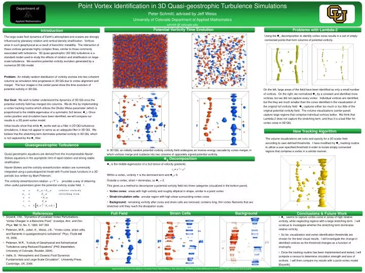
1. Point Vortex Identification in 3D Quasi-geostrophic Turbulence SimulationsPeter Schmitt; advised by Jeff WeissUniversity of Colorado Department of Applied Mathematicsschmitt @ colorado.edu Potential Vorticity Time Evolution Problems with Lambda-2 Introduction Using the  decomposition to identify vortex cores results in a set of simply connected points that form columns of potential vorticity. The large-scale fluid dynamics of Earth’s atmosphere and oceans are strongly influenced by planetary rotation and vertical density stratification. Vortices arise in such geophysical as a result of baroclinic instability. The interaction of these vortices generate highly complex flows, similar to those commonly associated with turbulence. 3D quasi-geostrophic (3D QG) turbulence is a standard model used to study the effects of rotation and stratification on large-scale turbulence. We examine potential vorticity evolution generated by a numerical 3D QG model. Problem: An initially random distribution of vorticity evolves into two coherent columns as simulation time progresses in 3D QG due to vortex alignment and merger. The four images in the center panel show the time evolution of potential vorticity in 3D QG. Our Goal: We wish to better understand the dynamics of 3D QG once the potential vorticity field has merged into columns. We do this by implementing a vortex tracking routine which utilizes the Okubo-Weiss parameter (which is proportional to the middle eigenvalue of a symmetric 3x3 tensor, ). Once vortex position and circulation have been identified, we will compare our results to a 3D point-vortex model. Initial results show that while works well as a filter in 2D QG turbulence simulations, it does not appear to serve as an adequate filter in 3D QG. We believe that the stretching term dominates potential vorticity in 3D QG, which is not captured by the  filter. On the left, large areas of the field have been identified as only a small number of vortices. On the right, we normalized  by a constant and identified more vortices, but we did not capture every vortex. Individual vortices are identified, but the they are much smaller than the cores identified in the visualization of the original full vorticity field.  captures either too much or too little of the original potential vorticity field. The volume visualizations (center panel) capture large regions that comprise individual vortices better. We think that Lambda-2 does not capture the stretching term, and thus it is a bad filter for vortex cores in 3D QG. New Tracking Algorithm The volume visualizations set color and opacity for a 3D scalar field according to user-defined thresholds. I have modified my  tracking routine to utilize a user-specified threshold in order to locate simply connected regions that comprise a vortex in a similar manner. Quasigeostrophic Turbulence In 3D QG, an initially random potential vorticity vorticity field undergoes an inverse energy cascade by vortex merger, in which vortices merge and coalesce into two columns of oppositely signed potential vorticity. Quasi-geostrophic equations are derived from the incompressible Navier-Stokes equations in the asymptotic limit of rapid rotation and strong stable stratification. Navier-Stokes and the vorticity-streamfunction relation are numerically integrated using a pseudospectral model with Fourier basis functions in a 3D periodic box written by Mark Petersen. The vorticity-streamfunction relation provides a way of obtaining other useful parameters given the potential vorticity scalar field, .  Decomposition •  is the middle eigenvector of a 3x3 tensor of velocity gradients. • Within a vortex, vorticity is the dominant term and < 0 • Outside a vortex, strain  dominates, so  > 0. • This gives us a method to decompose a potential vorticity field into three categories (visualized in the bottom panel). • Vortex cores: areas with high vorticity and roughly elliptical in shape, similar to a point vortex • Strain/circulation cells: annular region with high shear surrounding vortex cores • Background: remaining vorticity after cores and strain cells are removed; contains long, thin vortex filaments that are stretched until they reach the dissipation scale. References Strain Cells Background Conclusions & Future Work Full Field • Gryanik, V.M., “Dynamics of Localized Vortex Perturbations - ‘Vortex Charges’ in a Baroclinic Fluid,” Izvestiya, Atm. and Ocn. Phys.Vol 19, No. 5, 1983: 347-352 • Petersen, M.R., Julien, K., Weiss, J.B., “Vortex cores, strain cells, and filaments in quasigeostrophic turbulence” Phys. Fluidsvol 18, 2006. • Petersen, M.R., “A study of Geophysical and Astrophysical Turbulence using Reduced Equations” (PhD dissertation, University of Colorado, Boulder, 2004). • Vallis, G. “Atmospheric and Oceanic Fluid Dynamics: Fundamentals and Large-Scale Circulation”. University Press, Cambridge, UK, 2006. • seems to capture vortex cores in areas of high relative vorticity, while neglecting regions with a large stretching term. I will continue to investigate whether the stretching term dominates relative vorticity. • So far, visualization and vortex identification thresholds are chosen for the best visual results. I will investigate the change in identified vortices as the threshold changes as a function of enstrophy. • Once the tracking routine has been implemented and tested, I will compute a census to determine circulation strength and size of vortices. I will then compare my results with a point-vortex model [Gryanik]. Special thanks to Seth Claudepierre, Fernando Perez, Mark Petersen, Stan Solomon, Jeff Weiss and Mike Wiltberger for their support which made this work possible!